


Note
Click here to download the full example code
Spatial Transformer Networks Tutorial
Author: Ghassen HAMROUNI
In this tutorial, you will learn how to augment your network using a visual attention mechanism called spatial transformer networks. You can read more about the spatial transformer networks in the DeepMind paper
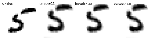
Spatial transformer networks are a generalization of differentiable attention to any spatial transformation. Spatial transformer networks (STN for short) allow a neural network to learn how to perform spatial transformations on the input image in order to enhance the geometric invariance of the model. For example, it can crop a region of interest, scale and correct the orientation of an image. It can be a useful mechanism because CNNs are not invariant to rotation and scale and more general affine transformations.
One of the best things about STN is the ability to simply plug it into any existing CNN with very little modification.
# License: BSD
# Author: Ghassen Hamrouni

from __future__ import print_function
import torch
import torch.nn as nn
import torch.nn.functional as F
import torch.optim as optim
import torchvision
from torchvision import datasets, transforms
import matplotlib.pyplot as plt
import numpy as np

plt.ion()   # interactive mode
Loading the data
In this post we experiment with the classic MNIST dataset. Using a standard convolutional network augmented with a spatial transformer network.
device = torch.device("cuda" if torch.cuda.is_available() else "cpu")

# Training dataset
train_loader = torch.utils.data.DataLoader(
    datasets.MNIST(root='.', train=True, download=True,
                   transform=transforms.Compose([
                       transforms.ToTensor(),
                       transforms.Normalize((0.1307,), (0.3081,))
                   ])), batch_size=64, shuffle=True, num_workers=4)
# Test dataset
test_loader = torch.utils.data.DataLoader(
    datasets.MNIST(root='.', train=False, transform=transforms.Compose([
        transforms.ToTensor(),
        transforms.Normalize((0.1307,), (0.3081,))
    ])), batch_size=64, shuffle=True, num_workers=4)
Out:
Downloading http://yann.lecun.com/exdb/mnist/train-images-idx3-ubyte.gz to ./MNIST/raw/train-images-idx3-ubyte.gz
Extracting ./MNIST/raw/train-images-idx3-ubyte.gz to ./MNIST/raw
Downloading http://yann.lecun.com/exdb/mnist/train-labels-idx1-ubyte.gz to ./MNIST/raw/train-labels-idx1-ubyte.gz
Extracting ./MNIST/raw/train-labels-idx1-ubyte.gz to ./MNIST/raw
Downloading http://yann.lecun.com/exdb/mnist/t10k-images-idx3-ubyte.gz to ./MNIST/raw/t10k-images-idx3-ubyte.gz
Extracting ./MNIST/raw/t10k-images-idx3-ubyte.gz to ./MNIST/raw
Downloading http://yann.lecun.com/exdb/mnist/t10k-labels-idx1-ubyte.gz to ./MNIST/raw/t10k-labels-idx1-ubyte.gz
Extracting ./MNIST/raw/t10k-labels-idx1-ubyte.gz to ./MNIST/raw
Processing...
Done!
Depicting spatial transformer networks
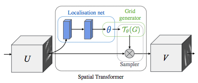
Spatial transformer networks boils down to three main components :
The localization network is a regular CNN which regresses the transformation parameters. The transformation is never learned explicitly from this dataset, instead the network learns automatically the spatial transformations that enhances the global accuracy.
The grid generator generates a grid of coordinates in the input image corresponding to each pixel from the output image.
The sampler uses the parameters of the transformation and applies it to the input image.
Note
We need the latest version of PyTorch that contains affine_grid and grid_sample modules.
class Net(nn.Module):
    def __init__(self):
        super(Net, self).__init__()
        self.conv1 = nn.Conv2d(1, 10, kernel_size=5)
        self.conv2 = nn.Conv2d(10, 20, kernel_size=5)
        self.conv2_drop = nn.Dropout2d()
        self.fc1 = nn.Linear(320, 50)
        self.fc2 = nn.Linear(50, 10)

        # Spatial transformer localization-network
        self.localization = nn.Sequential(
            nn.Conv2d(1, 8, kernel_size=7),
            nn.MaxPool2d(2, stride=2),
            nn.ReLU(True),
            nn.Conv2d(8, 10, kernel_size=5),
            nn.MaxPool2d(2, stride=2),
            nn.ReLU(True)
        )

        # Regressor for the 3 * 2 affine matrix
        self.fc_loc = nn.Sequential(
            nn.Linear(10 * 3 * 3, 32),
            nn.ReLU(True),
            nn.Linear(32, 3 * 2)
        )

        # Initialize the weights/bias with identity transformation
        self.fc_loc[2].weight.data.zero_()
        self.fc_loc[2].bias.data.copy_(torch.tensor([1, 0, 0, 0, 1, 0], dtype=torch.float))

    # Spatial transformer network forward function
    def stn(self, x):
        xs = self.localization(x)
        xs = xs.view(-1, 10 * 3 * 3)
        theta = self.fc_loc(xs)
        theta = theta.view(-1, 2, 3)

        grid = F.affine_grid(theta, x.size())
        x = F.grid_sample(x, grid)

        return x

    def forward(self, x):
        # transform the input
        x = self.stn(x)

        # Perform the usual forward pass
        x = F.relu(F.max_pool2d(self.conv1(x), 2))
        x = F.relu(F.max_pool2d(self.conv2_drop(self.conv2(x)), 2))
        x = x.view(-1, 320)
        x = F.relu(self.fc1(x))
        x = F.dropout(x, training=self.training)
        x = self.fc2(x)
        return F.log_softmax(x, dim=1)


model = Net().to(device)
Training the model
Now, let’s use the SGD algorithm to train the model. The network is learning the classification task in a supervised way. In the same time the model is learning STN automatically in an end-to-end fashion.
optimizer = optim.SGD(model.parameters(), lr=0.01)


def train(epoch):
    model.train()
    for batch_idx, (data, target) in enumerate(train_loader):
        data, target = data.to(device), target.to(device)

        optimizer.zero_grad()
        output = model(data)
        loss = F.nll_loss(output, target)
        loss.backward()
        optimizer.step()
        if batch_idx % 500 == 0:
            print('Train Epoch: {} [{}/{} ({:.0f}%)]\tLoss: {:.6f}'.format(
                epoch, batch_idx * len(data), len(train_loader.dataset),
                100. * batch_idx / len(train_loader), loss.item()))
#
# A simple test procedure to measure STN the performances on MNIST.
#


def test():
    with torch.no_grad():
        model.eval()
        test_loss = 0
        correct = 0
        for data, target in test_loader:
            data, target = data.to(device), target.to(device)
            output = model(data)

            # sum up batch loss
            test_loss += F.nll_loss(output, target, size_average=False).item()
            # get the index of the max log-probability
            pred = output.max(1, keepdim=True)[1]
            correct += pred.eq(target.view_as(pred)).sum().item()

        test_loss /= len(test_loader.dataset)
        print('\nTest set: Average loss: {:.4f}, Accuracy: {}/{} ({:.0f}%)\n'
              .format(test_loss, correct, len(test_loader.dataset),
                      100. * correct / len(test_loader.dataset)))
Visualizing the STN results
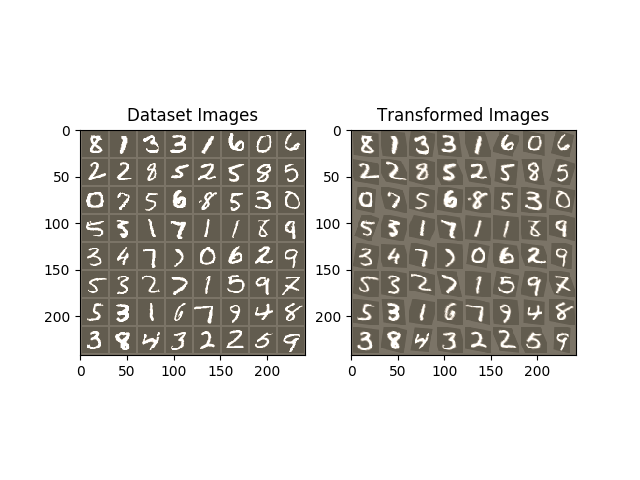
Now, we will inspect the results of our learned visual attention mechanism.
We define a small helper function in order to visualize the transformations while training.
def convert_image_np(inp):
    """Convert a Tensor to numpy image."""
    inp = inp.numpy().transpose((1, 2, 0))
    mean = np.array([0.485, 0.456, 0.406])
    std = np.array([0.229, 0.224, 0.225])
    inp = std * inp + mean
    inp = np.clip(inp, 0, 1)
    return inp

# We want to visualize the output of the spatial transformers layer
# after the training, we visualize a batch of input images and
# the corresponding transformed batch using STN.


def visualize_stn():
    with torch.no_grad():
        # Get a batch of training data
        data = next(iter(test_loader))[0].to(device)

        input_tensor = data.cpu()
        transformed_input_tensor = model.stn(data).cpu()

        in_grid = convert_image_np(
            torchvision.utils.make_grid(input_tensor))

        out_grid = convert_image_np(
            torchvision.utils.make_grid(transformed_input_tensor))

        # Plot the results side-by-side
        f, axarr = plt.subplots(1, 2)
        axarr[0].imshow(in_grid)
        axarr[0].set_title('Dataset Images')

        axarr[1].imshow(out_grid)
        axarr[1].set_title('Transformed Images')

for epoch in range(1, 20 + 1):
    train(epoch)
    test()

# Visualize the STN transformation on some input batch
visualize_stn()

plt.ioff()
plt.show()
Out:
Train Epoch: 1 [0/60000 (0%)]   Loss: 2.350204
Train Epoch: 1 [32000/60000 (53%)]      Loss: 0.691158

Test set: Average loss: 0.2023, Accuracy: 9402/10000 (94%)

Train Epoch: 2 [0/60000 (0%)]   Loss: 0.463056
Train Epoch: 2 [32000/60000 (53%)]      Loss: 0.313888

Test set: Average loss: 0.1185, Accuracy: 9630/10000 (96%)

Train Epoch: 3 [0/60000 (0%)]   Loss: 0.279039
Train Epoch: 3 [32000/60000 (53%)]      Loss: 0.332558

Test set: Average loss: 0.0930, Accuracy: 9699/10000 (97%)

Train Epoch: 4 [0/60000 (0%)]   Loss: 0.317962
Train Epoch: 4 [32000/60000 (53%)]      Loss: 0.157762

Test set: Average loss: 0.0760, Accuracy: 9775/10000 (98%)

Train Epoch: 5 [0/60000 (0%)]   Loss: 0.271342
Train Epoch: 5 [32000/60000 (53%)]      Loss: 0.145738

Test set: Average loss: 0.1344, Accuracy: 9569/10000 (96%)

Train Epoch: 6 [0/60000 (0%)]   Loss: 0.522058
Train Epoch: 6 [32000/60000 (53%)]      Loss: 0.369435

Test set: Average loss: 0.0611, Accuracy: 9809/10000 (98%)

Train Epoch: 7 [0/60000 (0%)]   Loss: 0.264292
Train Epoch: 7 [32000/60000 (53%)]      Loss: 0.076945

Test set: Average loss: 0.0587, Accuracy: 9819/10000 (98%)

Train Epoch: 8 [0/60000 (0%)]   Loss: 0.105667
Train Epoch: 8 [32000/60000 (53%)]      Loss: 0.327709

Test set: Average loss: 0.0533, Accuracy: 9829/10000 (98%)

Train Epoch: 9 [0/60000 (0%)]   Loss: 0.064149
Train Epoch: 9 [32000/60000 (53%)]      Loss: 0.169669

Test set: Average loss: 0.0604, Accuracy: 9807/10000 (98%)

Train Epoch: 10 [0/60000 (0%)]  Loss: 0.200340
Train Epoch: 10 [32000/60000 (53%)]     Loss: 0.073255

Test set: Average loss: 0.0549, Accuracy: 9832/10000 (98%)

Train Epoch: 11 [0/60000 (0%)]  Loss: 0.191361
Train Epoch: 11 [32000/60000 (53%)]     Loss: 0.020362

Test set: Average loss: 0.0455, Accuracy: 9864/10000 (99%)

Train Epoch: 12 [0/60000 (0%)]  Loss: 0.081118
Train Epoch: 12 [32000/60000 (53%)]     Loss: 0.106922

Test set: Average loss: 0.0490, Accuracy: 9857/10000 (99%)

Train Epoch: 13 [0/60000 (0%)]  Loss: 0.050231
Train Epoch: 13 [32000/60000 (53%)]     Loss: 0.154120

Test set: Average loss: 0.0415, Accuracy: 9876/10000 (99%)

Train Epoch: 14 [0/60000 (0%)]  Loss: 0.154015
Train Epoch: 14 [32000/60000 (53%)]     Loss: 0.022742

Test set: Average loss: 0.0392, Accuracy: 9874/10000 (99%)

Train Epoch: 15 [0/60000 (0%)]  Loss: 0.289922
Train Epoch: 15 [32000/60000 (53%)]     Loss: 0.049584

Test set: Average loss: 0.0383, Accuracy: 9884/10000 (99%)

Train Epoch: 16 [0/60000 (0%)]  Loss: 0.101700
Train Epoch: 16 [32000/60000 (53%)]     Loss: 0.100438

Test set: Average loss: 0.1181, Accuracy: 9658/10000 (97%)

Train Epoch: 17 [0/60000 (0%)]  Loss: 0.476445
Train Epoch: 17 [32000/60000 (53%)]     Loss: 0.089125

Test set: Average loss: 0.0375, Accuracy: 9892/10000 (99%)

Train Epoch: 18 [0/60000 (0%)]  Loss: 0.059651
Train Epoch: 18 [32000/60000 (53%)]     Loss: 0.118905

Test set: Average loss: 0.0384, Accuracy: 9877/10000 (99%)

Train Epoch: 19 [0/60000 (0%)]  Loss: 0.199291
Train Epoch: 19 [32000/60000 (53%)]     Loss: 0.095119

Test set: Average loss: 0.0358, Accuracy: 9887/10000 (99%)

Train Epoch: 20 [0/60000 (0%)]  Loss: 0.221594
Train Epoch: 20 [32000/60000 (53%)]     Loss: 0.019931

Test set: Average loss: 0.0386, Accuracy: 9877/10000 (99%)
Total running time of the script: ( 17 minutes 24.132 seconds)