Feature Construction for Reinforcement Learning in Hearts

Nathan R. Sturtevant and Adam M. White

Department of Computer Science

University of Alberta

Edmonton, AB, Canada T6G 2E8

{nathanst, awhite}@cs.ualberta.ca

Abstract.

Temporal difference (TD) learning has been used to learn strong evaluation functions in a variety of two-player games. TD-gammon illustrated how the combination of game tree search and learning methods can achieve grand-master level play in backgammon. In this work, we develop a player for the game of hearts, a 4-player game, based on stochastic linear regression and TD learning. Using a small set of basic game features we exhaustively combined features into a more expressive representation of the game state. We report initial results on learning with various combinations of features and training under self-play and against search-based players. Our simple learner was able to beat one of the best search-based hearts programs.

1 Introduction and Background

Learning algorithms have the potential to reduce the difficulty of building and tuning complex systems. But, there is often a significant amount of work required to tune each learning approach for specific problems and domains. We describe here the methods used to build a program to play the game of Hearts. This program is significantly stronger than a previously built expert-tuned program.

1.1 Hearts

Hearts is a trick-based card game, usually played with four players and a standard deck of 52 cards. Before play begins, 13 cards are dealt out to each player face-down. After all players look at their cards, the first player plays (leads) a card face-up on the table. The other players follow in order, if possible playing the same suit as was led. When all players have played, the player who played the highest card in the suit that was led wins or takes the trick. This player places the played cards face-down in his pile of taken tricks, and leads the next trick. This continues until all cards have been played.

The goal of Hearts is to take as few points as possible. A player takes points based on the cards in the tricks taken. Each card in the suit of hearts (♥) is worth one point, and the queen of spades (Q♠) is worth 13. If a player takes all 26 points, also called shooting the moon, they instead get 0 points, and the other players get 26 points each.

There are many variations on the rules of Hearts for passing cards between players before the game starts, determining who leads first, determining when you can lead hearts, and providing extra points based on play. In this work we use a simple variation of the rules: there is no passing of cards and no limitations on when cards can be played.

Hearts is an imperfect information game because players cannot see their opponents’ cards. Imperfect information in card games has been handled successfully using Monte-Carlo search, sampling possible opponent hands and solving them with perfect-information techniques. While there are known limitations of this approach [1], it has been quite effective in practice. The strongest bridge program, GIB [2], is based on Monte-Carlo search. This approach was also used for Hearts in Sturtevant’s thesis work [3]. Instead of learning to play the imperfect-information game of Hearts, we build a program that learns to play the perfect-information version of the game. We then use this as the basis for a Monte-Carlo player which plays the full game.

1.2 Hearts-Related Research

There have been several studies on learning and search algorithms for the game of Hearts. Because Hearts is a multi-player game (more than two players) minimax search cannot be used. Instead maxⁿ[4] is the general algorithm for playing multi-player games.

Perkins [5] developed two search-based approaches for multiplayer imperfect information games based on maxⁿsearch. The first search method built a maxⁿ tree based on move availability and value for each player. The second method maximized the maxⁿ value of search trees generated by Monte-Carlo. The resultant players yielded a low to moderate level of play against human and rule-based based players.

One of the strongest computer Hearts programs [3], uses efficient multi-player pruning algorithms coupled with Monte-Carlo search and a hand-tuned evaluation function. When tested against a well-known commercial program¹, it beat the program by 1.8 points per hand on average, and 20 points per game. The game of Hearts is not 'solved': this program is still weaker than humans. We used this program as an expert to train against in some of our experiments for this paper. For the remainder of this paper we will refer to the full program as the Imperfect Information Expert (IIE) and the underlying solver as the Perfect Information Expert (PIE).

One of the first applications of temporal difference (TD) learning methods to Hearts was by [6]. These results, however, are quite weak. The resulting program was able to beat a random program, and in a small competition out-played other learned players. But, it was unable to beat Monte-Carlo based players. Fujita et al have done several studies on applying reinforcement learning (RL) algorithms to the game of Hearts. In their recent work [7], Fujita et al modeled the game as a partially-observable Markov decision process (POMDP), where the agent can observe the game state, but other dimensions of the state, such as the opponents’ hands, are unobservable. Using a one step history, they constructed a new model of the opponents’ action selection heuristic according to the previous action selection models. Although their learned player performed better than their previous players and also beat rule-based players, it is difficult to know the true strength of the learning algorithm and resultant player. This is due to the limited number of training games and lack of validation of the final learned player. The work of Fujita et al differs from ours in that they understate the feature selection problem, which was a crucial factor in the high level of play exhibited by our learning agents.

Finally, Furnkranz et al [8] have done initial work using RL techniques to employ an operational advice system to play hearts. A neural network was used with TD learning to learn a mapping from state abstraction and action selection advice to a number of move selection heuristics. This allowed their system to learn a policy using a very small set of features (15) and little training. However, this work is still in its preliminary stages and the resulting player exhibited only minor improvement over the greedy action selection of the operational advice system on which the learning system was built.

1.3 Reinforcement Learning

In reinforcement learning an agent interacts with an environment by selecting actions in various states to maximize the sum of scalar rewards given to it by the environment. In hearts, for example, a state consists of the cards held by and taken by each player in the game and negative reward is assigned each time you take a trick with points on it. The environment includes other players as well as the rules of the game.

The RL approach has strong links to the cognitive processes that occur in the brain and has proved effective in Robocup soccer [9], industrial elevator control [10] and backgammon [10]. These learning algorithms were able to obtain near optimal policies simply from trial and error interaction with the environment in high dimensional and sometimes continuous valued state and action spaces.

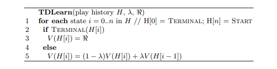
Fig. 1. Learning using TD(λ) given a history of game play

All of the above examples use TD learning [10]. In the simplest form of TD learning an agent stores a scalar value for the estimated reward of each state, V(s). The agent selects the action that leads to the state with the highest utility. In the tabular case, the value function is represented as an array indexed by states. At each decision point or step of an episode the agent updates the value function according to the observed rewards. TD uses bootstrapping, where an agent updates its state value with the reward received on the current time step and the difference between the current state value and the state value on the previous time step. TD(λ) updates all previously encountered state values according to an exponential decay, which is determined by λ. The pseudo-code for TD-learning used in this work is given in Figure 1, where His the history of game play and < is the reward (points taken) at the end of an episode.

1.4 Function Approximation

TD(λ) is guaranteed to converge to an optimal solution in the tabular case, where a unique value can be stored for every state. Many interesting problems, such as Hearts, have a restrictively large of number states. Given a deck of 52 cards with each player being dealt 13 cards, there are 52!/13!⁴ = 5.4 × 10²⁸ possible hands in the game. This is, in fact, only a lower bound on actual size of the state space because it does not consider the possible states that we could encounter while playing the game. Regardless, we cannot store this many states in memory, and even if we could, we do not have the time to visit and train in every state.

Therefore, we need some method to approximate the states of the game. In general this is done by choosing a set of features which approximate the states of the environment. A function approximator must map these features into a value function for each state in the environment. This generalizes learning over similar states and increases the speed of learning, but potentially introduces generalization error as the features will not represent the state space exactly.

One of the simplest function approximators is the linear perceptron. A perceptron computes a state value function as a weighted sum of its input features. Weights w are updated according to the formula:

w ← w + α·error_s·φ_s

given the current state s, current state output error error_s , which is provided by TD learning, and the features of the current state, φ_s .

Because output of a perceptron is a linear function of its input, it can only learn linearly separable functions. Most interesting problems require a nonlinear mapping from features to state values. In many cases one would use a more complex function approximator, such as neural networks, radial basis functions, CMAC tile coding or kernel based regression. These methods can represent a variety of nonlinear functions.An alternate approach, which we take, is to use a simple function approximator with more complicated set of features. We use linear function approximation for several reasons: Linear regression is easy to implement, the learning rate scales linearly with the number of features, and the learned network weights are easier to analyze. Our results demonstrate that a linear function approximation is able to learn and efficiently play the imperfect information game of Hearts.

We illustrate how additional features can allow a linear function approximator to solve a nonlinear task with a simple example: Consider the task of learning the XOR function based on two inputs. A two input perceptron cannot learn this function because XOR is not linearly separable. But, if we simply augment the network input with an extra input which is the logical AND of the first two inputs, the network can learn the optimal weights. In fact, all subsets of n points are always linearly separable in n − 1 dimensional space. Thus, given enough features, a non-linear problem can have a exact linear solution.

2 Learning to Play Hearts

Before describing our efforts for learning in Hearts, we examine the features of backgammon which make it an ideal domain for TD learning. In backgammon, pieces are always forced to move forward, except in the case of captures, so games cannot run forever. The set of moves available to each player are determined by a dice roll, which means that even from the same position the learning player may be forced to follow different lines of play each game, unlike in a deterministic game such as chess where the exact same game can easily be repeated. Thus, self-play has worked well in backgammon.

Hearts has some similar properties. Each player makes exactly 13 moves in every game, which means we do not have to wait long to get exact rewards associated with play. Thus, we can quickly generate and play large numbers of training games. Additionally, cards are dealt randomly, so, like in backgammon, players are forced to explore different lines of play in each game. Another useful characteristic of Hearts is that even a weak player occasionally gets good cards. Thus, we are guaranteed to see examples of good play.

One key difference between Hearts and backgammon is that the value of board positions in backgammon tend to be independent. In Hearts, however, the value of any card is relative to what other cards have been played. For instance, it is a strong move to play the 10♥ when the 2-9♥ have already been played. But, if they have not been played, it is a weak move. This complicates the features needed to play the game.

2.1 Feature Generation

Given that we are using a simple function approximator, we need a rich set of features. In the game of Hearts, and card games in general, there are many very simple features which are readily accessible. For instance, we can have a single binary feature for each card that each player holds in their hand and for each card that they have taken (e.g. the first feature is true if Player 1 has the 2♥, the second is true if Player 1 has the 3♥, etc.). This would be a total of 104 features for each player and 416 total features for all players. This set of features fully specifies a game, so in theory it should be sufficient for learning, given a suitably powerful function approximator and learning algorithm.

However, consider a simple question like: “Does player 1 has the lowest heart left?” Answering this question based on such simple features is quite difficult, because the lowest heart is determined by the cards that have been played already. If we wanted to express this given the simple features described above, it would look something like: “[Player 1 has the 2♥] OR [Player 1 has the 3♥AND Player 2 does not have the 2♥AND Player 3 does not have the 2♥AND Player 4 does not have the 2♥] OR [Player 1 has the 4♥ ...]”. While this full combination could be learned by a non-linear function approximator, it is unlikely to be.

Another approach for automatically combining basic game features is GLEM [11]. GLEM measures the significance of groups of basic features, building mutually exclusive sets for which weights are learned. This approach is well-suited for many board games. But, as we demonstrated above, the features needed to play a card game well are quite complex and not easily learnable. Similar principles may be used to refine our approach, but we have yet to consider them in detail.

Our approach is to define a set of useful features, which we will call atomic features. These features are perfect-information features, so they depend on the cards other players hold. Then we built higher level features by combining these atomic features together. One set of atomic features used for learning can be found in Appendix A.

Attempting to manually build all useful combinations of the atomic features would be tedious, error-prone, and time consuming. Instead, we take a more brute-force approach. Given a set of atomic features, we generate new features by exhaustively taking all pair-wise AND combinations of the atomic features. Obviously we could take this further by adding OR operations and negations. But, to limit feature growth we currently only consider the AND operator.

2.2 Learning Parameters

For all experiments described here we used TD-learning as follows. The value of λ was set to 0.75. We first generated and played out a game of Hearts using a single learning player and either three expert search players taken from Sturtevant's thesis work [3] (PIE and IIE), or three copies of our learned network for self-play. In most experiments we report results of playing the hand-tuned evaluation function (PIE) against the learned network, without Monte-Carlo. Thus, the expert player’s search and evaluation function took full advantage of the perfect information provided (player's hands) and is a fair opponent for our perfect information learning player. Moves were selected using the maxⁿalgorithm with a lookahead depth of one to four, based on how many cards were left to play on the current trick. When backing up values in the search tree, we used our own network as the evaluation function for our opponents.

To simplify the learned network we only evaluated the game in states where there were no cards on the current trick. We did not learn in states where all the points had already been played. After playing a game we computed the reward for the learning player and then stepped backwards through the game, using TD-learning to update our target output and train our perceptron to predict the target output at each step. We did not attempt to train using more complicated methods such as TDLeaf [12].

2.3 Learning To Avoid the Q♠

Our first learning task was to predict whether we would take the Q♠. We trained the perceptron to return an output between 0 and 13, the value of the Q♠ in the game. In practice, we cut the output off with a lower bound of 0 + ℰ and an upper bound of 13 − ℰ so that the search algorithm could always distinguish between states where we expected to take the Q♠versus states where we already had taken the Q♠, preferring those where we had not yet taken the queen. The perceptron learning rate was set to 1/(13 × number active features).

We used 60 basic features, listed in Appendix A, as the atomic features for the game. Then, we built pair-wise, three-wise and four-wise combinations of these atomic features. The pair-wise combinations of these features results in 1,830 total features, three-wise combinations of the atomic features results in 34,280 total features, and four-wise combinations of features results in 523,685 total features. But, many of these features are mutually exclusive and can never occur. We initialized the feature weights randomly between ± 1/numfeatures.

Fig. 2. Learning to not take the Q♠ using various combinations of atomic features. The break-even point is at 3.25

The average score of the learning player during training is shown in Figure 2. This learning curve is performance relative to PIE. Except for the four-wise features, we did five training runs of 200,000 games against the expert program. Scores were then averaged between each run and over a 5,000 game window. With 13 points in each hand, evenly matched players would expect to take 3.25 points per hand. The horizontal line in the figure indicates the break-even point between the learned and expert programs.

These results demonstrate that the atomic features alone were insufficient for learning to avoid taking the Q♠. The pair-wise and three-wise features were also insufficient, but are better than the atomic features alone. The four-wise combinations of features, however, are sufficient to beat the expert program.

Table 1. Features predicting we can avoid the Q♠.

Table 2. Features predicting we will take the Q♠.

The features which best predict avoiding the Q♠ are shown in Table 1. This player actually uses all atomic, pair-wise, three-wise and four-wise features, so some of the best features in this table only have three atomic features. Weights are negative because they reduce our expected score in the game.

There are a few things to note about these features. First, we can see that the highest weighted feature is also one learned quickly by novice players: If the player with the Q♠ has no other spades and we can lead spades, we are guaranteed not to take the Q♠. In this case, leading a spade will force the Q♠ onto another player.

Because we have generated all four-wise combinations of features, and this feature only requires three atomic features to specify, we end up getting the same atomic features repeated multiple times with an extra atomic features added. The features ranked 2, 4 and 5 are copies of the first feature with one extra atomic feature added. The 148th ranked feature should seem odd, but we will explain it when looking at the features that predict that we will take the Q♠.

The features that best predict taking the Q♠ are found in Table 2. These features are slightly less intuitive. We might expect to find symmetric versions of the features from Table 1 in Table 2 (eg. we have a single Q♠ and the player to lead has spades). This feature is among the top 300 (out of over 500,000) features, but not in the top five features.

What is interesting about Table 2 is the interactions between features. Again, we see that the atomic features which make up the 2nd ranked feature are a subset of the highest ranked feature. In fact, these two atomic features appear 259 times in the top 20,000 features. They appear 92 times as part of a feature which decreases the chance of us taking the Q♠, while 167 times they increase the likelihood. We can use this to explain what has been learned: Having the Q♠ with only one other spade in our hand means we are likely to take the Q♠ (feature 2 in Table 2). If we also have the lead (feature 1 in Table 2), we are even more likely to take the Q♠. But, if someone else has the lead, and they do not have spades (feature 148 in Table 1), we are much less likely to take the Q♠.

The ability to do this analysis is one of the benefits of putting the complexity into the features instead of the function approximator. If we rely on a more complicated function approximator to learn weights, it is very difficult to analyze the resulting network. Because we have simple weights on more complicated features it is much easier to analyze what has been learned.

2.4 Learning to Avoid Hearts

We used similar methods to predict how many hearts we would take within a game, and learned this independently of the Q♠. One important difference between the Q♠ and points taken from hearts is that the Q♠ is taken by one player all at once, while hearts are gradually taken throughout the course of the game. To handle this, we removed 14 Q♠specific features and added 42 new atomic features to the 60 atomic features used for learning the Q♠. The new features were the number of points (0-13) taken by ourselves, the number of points taken (0-13) by all of our opponents combined, and the number of points (0-13) left to be taken in the game.

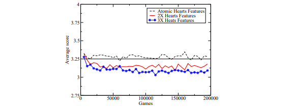
Fig. 3. Learning to not take the Hearts using various combinations of atomic features

Given these atomic features, we then trained with the atomic (88), pair- wise (3,916) and three-wise (109,824) combinations of features. As before, we present the results averaged over five training runs (200,000 games each) and then smoothed over a window of 5,000 games. The learning graph for this train- ing is in Figure 3. An interesting feature of these curves is that, unlike learning the Q♠, we are already significantly beating the expert with the two-wise features set. It appears that learning to avoid taking hearts is a bit easier than avoiding the Q♠. However, when we go from two-wise to three-wise features, the increase in performance is much less. Because of this, we did not try all four-wise combinations of features.

2.5 Learning Both Hearts and the Q♠

Given two programs that separately learned partial components of the full game of Hearts, the final task is to combine them together. We did this by extracting the most useful features learned in each separate task, and then combined them to learn to play the full game. The final learning program used the top 2,000 features from learning to avoid hearts and the top 10,000 features used when learning to avoid the Q♠.

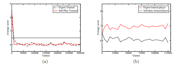
Fig. 4. (a) Performance of expert-trained and self-trained player against the expert. (b) Performance of self-trained and expert-trained programs against each other.

We tried training this program in two ways: first, by playing against PIE, and second, by self-play. During this training shooting the moon was disabled. The first results are plotted in Figure 4(a). Instead of plotting the learning curve, which is uninteresting for self-play, we instead plot the performance of the learned network against the expert program. We did this by playing games between the networks that were saved during training and the expert program. For two player types there are 16 ways to place those types into a four-player game, however two of these ways contain all learning or all expert players. 100 games were played for each of the 14 possible arrangements for a total of 1400 hands played for each data point in the curve. There are 26 points in the full game, so the break-even point, indicated by a horizontal line, falls at 6.5 points. Both the self-trained player and the expert-trained player learn to beat the expert by the same rate, about 1 point per hand.

In Figure 4(b) we show the results from taking corresponding networks trained by self-play and expert-play and playing them in tournaments against each other. (Again, 1400 games for each player type.) Although both of these programs beat PIE program by the same margin, the program trained by self play managed to beat PIE by a large margin; again about 1 point per hand.

While we cannot provide a decisive explanation for why this occurs, we speculate that the player which only trains against the expert does not sufficiently explore different lines of play, and so does not learn to play well in certain situations of the game where the previous expert always made mistakes. The program trained by self-play, then, is able to exploit this weakness.

2.6 Imperfect Information Play

Given the learned perfect-information player, we then played it against IIE. For these tests, shooting the moon was enabled. Both programs used 20 Monte-Carlo models and analyzed the first trick of the game in each model (up to 4-ply). When just playing single hands, the learned player won 56.9% of the hands with an average score of 6.35 points per hand, while the previous expert program averaged 7.30 points per hand. When playing full games (repeated hands to 100 points), the learned player won 63.8% of the games with an average score of 69.8 points per game as opposed to 81.1 points per game for IIE.

3 Conclusions and Future Work

The work presented in this paper presents a significant step in learning to play the game of Hearts and in learning for multi-player games in general. We have shown that a search-based player with a learned evaluation function can learn to play Hearts using a simple linear function approximator and TD-learning with either expert-based training or self-play. Furthermore, our learned player beat one of the best-known programs in the world in the imperfect information version of Hearts.

There are several areas of interest for future research. First, we would like to extend this work to the imperfect information game to see if the Monte-Carlo based player can be beat. Next, there is a question of the search algorithm used for training and play. There are weaknesses in maxⁿanalysis that soft-maxⁿ[13] addresses; the paranoid algorithm [14] could be used as well.

Our ultimate goal is to play the full game of Hearts well at an expert level, which includes passing cards between players and learning to prevent other play-ers from shooting the moon. It is unclear if just learning methods can achieve this or if other specialized algorithms may be used to tasks such as shooting the moon. But, this work is the first step in this direction.

Acknowledgments

We would like to thank Rich Sutton, Mark Ring and Anna Koop for their feedback and suggestions regarding this work. This work was supported by Alberta’s iCORE, the Alberta Ingenuity Center for Machine Learning and NSERC.

A Atomic Features Used to Learn the Q♠

Unless explicitly stated, all features refer to cards in our hand. The phrase “to start” refers to the initial cards dealt. “Exit” means we have a card guaranteed not to take a trick. “Short” means we have no cards in a suit. “Backers” are the J-2♠. “Leader” and “Q♠player” refers to another player besides ourself.