1 . Introduction
Deep neural networks have become the de facto model for computer vision applications. Their success is partially attributable to their apparent scalability, i.e., the empirical observation that training them on larger datasets produces better performance [25, 17, 35, 46, 34, 18]. Deep networks often achieve their strong performance through supervised learning, which requires a labeled dataset. The performance benefit conferred by the use of a larger dataset can therefore come at a significant cost since labeling data often requires human labor. This cost can be particularly extreme when labeling must be done by an expert (for example, a doctor in medical applications).
A powerful approach for training models on a large amount of data without requiring a large amount of labels is semi-supervised learning (SSL). SSL mitigates the requirement for labeled data by providing a means of leveraging unlabeled data. Since unlabeled data can often be obtained with minimal human labor, any performance boost conferred by SSL often comes with low cost. This has led to a plethora of SSL methods that are designed for deep networks [28, 39, 21, 43, 3, 45, 2, 22, 38].
A popular class of SSL methods can be roughly viewed as producing an artificial label for each unlabeled image and then training the model to predict the artificial label when fed the unlabeled image as input. For example, pseudo-labeling [22] (also called self-training [27, 46, 37, 40]) uses the model’s class prediction as a label to train against. Similarly, consistency regularization [39, 21] obtains an artificial label using the model’s predicted distribution after randomly modifying the input or model function.
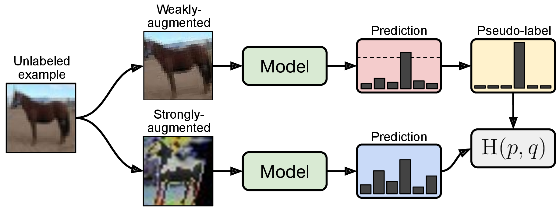
In this work, we continue the trend of recent state-of-the-art methods that combine diverse mechanisms for producing artificial labels [3, 45, 2, 28]. We introduce FixMatch, which produces artificial labels using both consistency regularization and pseudo-labeling. Crucially, the artificial label is produced based on a weakly-augmented unlabeled image (e.g., using only flip-and-shift data augmentation) which is used as a target when the model is fed a strongly-augmented version of the same image. Inspired by UDA [45] and ReMixMatch [2], we leverage CutOut [13], CTAugment [2], and RandAugment [10] for strong augmentation, which all produce heavily distorted versions of a given image. Following the approach of pseudo-labeling [22], we only retain an artificial label if the model assigns a high probability to one of the possible classes. A diagram of FixMatch is shown in fig. 1.
While FixMatch comprises a simple combination of existing techniques, we nevertheless show that it obtains state-of-the-art performance on the most commonly-studied SSL benchmarks. For example, FixMatch achieves 94.93% accuracy on CIFAR-10 with 250 labeled examples compared to the previous state-of-the-art of 93.73% [2] in the standard experimental setting from [31]. We also explore the limits of our approach by applying it in the extremely-scarce-labels regime, obtaining 88.61% accuracy on CIFAR-10 with only 4 labels per class. Since FixMatch is similar to existing approaches but achieves substantially better performance, we include an extensive ablation study to determine which factors contribute the most to its success. Our ablation study also includes basic experimental choices that are often ignored or not reported when new SSL methods are proposed (such as the optimizer or learning rate schedule) because we found that they can have an outsized impact on performance.
In the following section, we introduce FixMatch and the ideas it builds upon. In section 3, we discuss how FixMatch relates to existing SSL algorithms. Section 4 and section 5 include our experimental results and ablation study, respectively. Finally, we conclude in section 6 with a summary and an outlook on future work.
2 . FixMatch
Overall, the FixMatch algorithm is a simple combination of two common approaches to SSL: Consistency regularization and pseudo-labeling. Its main novelty comes from the combination of these two ingredients as well as the use of a separate weak and strong augmentation when performing consistency regularization. In this section, we first review consistency regularization and pseudo-labeling before describing the FixMatch algorithm in detail. We also describe the other factors, such as regularization, which contribute to FixMatch’s empirical success.
For an L-class classification problem, let us define
𝒳 =  (xb,pb) : b ∈ (1,…,B)
 a batch of B labeled examples,
where xb are the training examples and pb are one-hot labels.
Let 𝒰 =
a batch of B labeled examples,
where xb are the training examples and pb are one-hot labels.
Let 𝒰 =  ub : b ∈ (1,…,μB)
 be a batch of μB unlabeled
examples where μ is a hyperparameter that determines the
relative sizes of 𝒳 and 𝒰. Let pm(y∣x) be the predicted class
distribution produced by the model for input x. We denote the
cross-entropy between two probability distributions p and q as
H(p,q). We perform two types of augmentations as part of
FixMatch: strong and weak, denoted by 𝒜(⋅) and α(⋅)
respectively. We describe the form of augmentation we use for
𝒜 and α in section 2.3.
be a batch of μB unlabeled
examples where μ is a hyperparameter that determines the
relative sizes of 𝒳 and 𝒰. Let pm(y∣x) be the predicted class
distribution produced by the model for input x. We denote the
cross-entropy between two probability distributions p and q as
H(p,q). We perform two types of augmentations as part of
FixMatch: strong and weak, denoted by 𝒜(⋅) and α(⋅)
respectively. We describe the form of augmentation we use for
𝒜 and α in section 2.3.
2.1 . Background
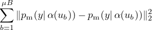
Consistency regularization is an important component of many recent state-of-the-art SSL algorithms. Consistency regularization utilizes unlabeled data by relying on the assumption that the model should output similar predictions when fed perturbed versions of the same image. This idea was first proposed in [39, 21], where the model is trained both via a standard supervised classification loss and on unlabeled data via the loss function
 | (1) |
Note that both α and pm are stochastic functions, so the two terms in eq. (1) will indeed have different values. Extensions to this idea include using an adversarial transformation in place of α [28], using a running average or past model predictions for one invocation of pm in eq. (1) [43, 21], using a cross-entropy loss in place of the squared ℓ2 loss [28, 45, 2], using stronger forms of augmentation [45, 2], and using consistency regularization as a component in a larger SSL pipeline [3, 2].
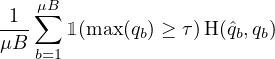
Pseudo-labeling leverages the idea that we should use the model itself to obtain artificial labels for unlabeled data. This idea was introduced decades ago [27, 40]. Pseudo-labeling specifically refers to the use of “hard” labels (i.e., the argmax of the model’s output) and only retaining artificial labels whose largest class probability fall above a predefined threshold [22]. Letting qb = pm(y|ub), pseudo-labeling uses the following loss function on unlabeled data:
 | (2) |
where qb=argmax(qb) and τ is the threshold hyperparameter. Note that for simplicity we assume that argmax applied to a probability distribution produces a valid “one-hot” probability distribution. The use of a hard label makes pseudo-labeling closely related to entropy minimization [16, 38], where the model’s predictions are encouraged to be low-entropy (i.e., high-confidence) on unlabeled data.
2.2 . Our Algorithm: FixMatch
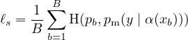
The loss function for FixMatch consists exclusively of two cross-entropy loss terms: a supervised loss ℓs applied to labeled data and an unsupervised loss ℓu. Specifically, ℓs is just the standard cross-entropy loss on weakly augmented labeled examples:
 | (3) |
For unlabeled data,1 FixMatch computes an artificial label for each example which is then used in a standard cross-entropy loss. To obtain an artificial label, we first compute the model’s predicted class distribution given a weakly-augmented version of a given unlabeled image: qb = pm(y∣α(ub)). Then, we use qb=argmax(qb) as a pseudo-label, except we enforce the cross-entropy loss against the model’s output for a strongly-augmented version of ub:
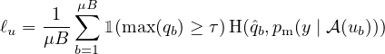 | (4) |
where τ is a scalar hyperparameter denoting the threshold above which we retain a pseudo-label. In sum, the loss minimized by FixMatch is simply ℓs + λuℓu where λu is a fixed scalar hyperparameter denoting the relative weight of the unlabeled loss. We present a complete algorithm for FixMatch in algorithm 1 of the supplementary material.
Note that eq. (4) is similar to the pseudo-labeling loss in eq. (2). The crucial difference is that the artificial label is computed based on a weakly-augmented image and the loss is enforced against the model’s output for a strongly-augmented image. This introduces a form of consistency regularization which, as we will show in section 5, is crucial to FixMatch’s success. We also note that it is typical in modern SSL algorithms to increase the weight of the unlabeled loss term (λu) over the training [43, 21, 3, 2, 31]. We found that this was unnecessary for FixMatch, which may be due to the fact that max(qb) is typically less than τ early in training. As training progresses, the model’s predictions become more confident and it is more frequently the case that max(qb) > τ. This suggests that pseudo-labeling may produce a natural curriculum “for free”. Similar justifications have been used in the past for ignoring low-confidence predictions in visual domain adaptation [14].
2.3 . Augmentation in FixMatch
FixMatch leverages two kinds of augmentations: “weak” and “strong”. In all of our experiments, weak augmentation is a standard flip-and-shift augmentation strategy. Specifically, we randomly flip images horizontally with a probability of 50% on all datasets except SVHN and we randomly translate images by up to 12.5% vertically and horizontally.
For “strong” augmentation, we experiment with two approaches which are based on AutoAugment [9]. AutoAugment learns an augmentation strategy based on transformations from the Python Imaging Library2 using reinforcement learning. This requires labeled data to learn the augmentation pipeline, making it problematic to use in SSL settings where limited labeled data is available. As a result, variants of AutoAugment have been proposed which do not require the augmentation strategy to be learned ahead of time with labeled data. We experiment with two such variants: RandAugment [10] and CTAugment [2]. Note that, unless otherwise stated, we use Cutout [13] followed by either of these strategies.
Given a collection of transformations (e.g., color inversion, translation, contrast adjustment, etc.), RandAugment randomly selects transformations for each sample in a mini-batch. As originally proposed, RandAugment uses a single fixed global magnitude that controls the severity of all distortions [10]. The magnitude is a hyperparameter that must be optimized on a validation set e.g., using grid search. We found that sampling a random magnitude from a pre-defined range at each training step (instead of using a fixed global value) works better for semi-supervised training, similar to what is used in UDA [45].
Instead of setting the transformation magnitudes randomly, CTAugment [2] learns them online over the course of training. To do so, a wide range of transformation magnitude values is divided into bins (as in AutoAugment [9]) and a weight (initially set to 1) is assigned to each bin. All examples are augmented with a pipeline consisting of two transformations which are sampled uniformly at random. For a given transformation, a magnitude bin is sampled randomly with a probability according to the (normalized) bin weights. To update the weights of the magnitude bins, a labeled example is augmented with two transformations whose magnitude bins are sampled uniformly at random. The magnitude bin weights are then updated according to how close the model’s prediction is to the true label. Further details on CTAugment can be found in [2].
2.4 . Additional important factors
Semi-supervised performance can be substantially impacted by factors other than the SSL algorithm used because considerations like the amount of regularization can be particularly important in the low-label regime. This is compounded by the fact that the performance of deep networks trained for image classification can heavily depend on the architecture, optimizer, training schedule, etc. These factors are typically not emphasized when new SSL algorithms are introduced. Instead of minimizing the importance of these factors, we endeavor to quantify their importance and highlight which ones have a significant impact on performance. Most of this analysis is performed in section 5. In this section we identify a few key considerations.
First, as mentioned above, we find that regularization is particularly important. In all of our models and experiments, we use simple weight decay regularization. We also found that using the Adam optimizer [19] resulted in worse performance and instead use standard SGD with momentum [42, 33, 29]. We did not find a substantial difference between standard and Nesterov momentum. For a learning rate schedule, we use a cosine learning rate decay [23] which sets the learning rate to
 | (5) |
where η is the initial learning rate, k is the current training step, and K is the total number of training steps. Note that this schedule effectively decays the learning rate from η to close to 0 by following a cosine curve. Finally, we report final performance using an exponential moving average of model parameters.
| Algorithm | Artificial label augmentation |
Prediction augmentation |
Artificial label post-processing | Notes |
| TS [39]/Π-Model [36] | Weak | Weak | None | |
| Temporal Ensembling [21] | Weak | Weak | None | Uses model from earlier in training |
| Mean Teacher [43] | Weak | Weak | None | Uses an EMA of parameters |
| Virtual Adversarial Training [28] | None | Adversarial | None | |
| UDA [45] | Weak | Strong | Sharpening | Ignores low-confidence artificial labels |
| MixMatch [3] | Weak | Weak | Sharpening | Averages multiple artificial labels |
| ReMixMatch [2] | Weak | Strong | Sharpening | Sums losses for multiple predictions |
| FixMatch | Weak | Strong | Pseudo-labeling |
3 . Related work
Semi-supervised learning is a mature field with a huge diversity of approaches. In this review of related work, we focus only on methods closely related to FixMatch. Broader introductions to the field are provided in [51, 52, 5].
The idea behind pseudo-labeling or self-training has been around for decades [40, 27]. The generality of self-training (i.e., using a model’s predictions to obtain artificial labels for unlabeled data) has led it to be been applied in a diversity of domains including NLP [26], object detection [37], image classification [22, 46], domain adaptation [53], to name a few. Pseudo-labeling refers to a specific variant where model predictions are converted to hard labels and are only retained when the classifier is sufficiently confident [22]. Some studies have suggested that pseudo-labeling is not competitive against other modern SSL algorithms on its own [31]. However, recent SSL algorithms have used pseudo-labeling as a part of their pipeline to produce better results [1, 32]. Similarly, as mentioned above, pseudo-labeling results in a form of entropy minimization [16] which has been used as a component for many powerful SSL techniques [28].
Consistency regularization was first proposed as “Regularization With Stochastic Transformations and Perturbations for Deep Semi-Supervised Learning” (Transformation/Stability or TS for short) [39] or the “Π-Model” [36]. Early extensions included using an exponential moving average of model parameters [43] or using previous model checkpoints [21] when producing artificial labels. A variety of methods have been used to produce random perturbations including data augmentation [14], stochastic regularization (e.g. Dropout [41]) [39, 21], and adversarial perturbations [28]. More recently, it has been shown that using strong data augmentation can produce better results [45, 2]. These heavily-augmented examples are almost certainly outside of the data distribution, which has in fact been shown to be potentially beneficial for SSL [11].
Of the aforementioned work, FixMatch bears the closest resemblance to two recent algorithms: Unsupervised Data Augmentation (UDA) [45] and ReMixMatch [2]. UDA and ReMixMatch both use a weakly-augmented example to generate an artificial label and enforce consistency against strongly-augmented examples. Neither of them use pseudo-labeling, but both approaches “sharpen” the artificial label to encourage the model to produce high-confidence predictions. UDA in particular also enforces consistency when the highest probability in the predicted class distribution for the artificial label is above a threshold. The thresholded pseudo-labeling of FixMatch has a similar effect to sharpening. In addition, ReMixMatch anneals the weight of the unlabeled data loss, which we omit from FixMatch because we posit that the thresholding used in pseudo-labeling has a similar effect (as mentioned in section 2.2). These similarities suggest that FixMatch can be viewed as a substantially simplified version of UDA and ReMixMatch, where we have combined two common techniques (pseudo-labeling and consistency regularization) while removing many components (sharpening, training signal annealing from UDA, distribution alignment and the rotation loss from ReMixMatch, etc.).
Since the core approach of FixMatch is a simple combination of two existing techniques, it also bears substantial similarities to many previously-proposed SSL algorithms. We provide a concise comparison of each of these techniques in table 1 where we list the augmentation used for the artificial label, the model’s prediction, and any post-processing applied to the artificial label. A more thorough empirical comparison of these different algorithms and their constituent approaches is provided in the following section.
| CIFAR-10 | CIFAR-100 | SVHN
| |||||||
| Method | 40 labels | 250 labels | 4000 labels | 400 labels | 2500 labels | 10000 labels | 40 labels | 250 labels | 1000 labels |
| Π-Model | - | 54.26±3.97 | 14.01±0.38 | - | 57.25±0.48 | 37.88±0.11 | - | 18.96±1.92 | 7.54±0.36 |
| Pseudo-Labeling | - | 49.78±0.43 | 16.09±0.28 | - | 57.38±0.46 | 36.21±0.19 | - | 20.21±1.09 | 9.94±0.61 |
| Mean Teacher | - | 32.32±2.30 | 9.19±0.19 | - | 53.91±0.57 | 35.83±0.24 | - | 3.57±0.11 | 3.42±0.07 |
| MixMatch | 47.54±11.50 | 11.05±0.86 | 6.42±0.10 | 67.61±1.32 | 39.94±0.37 | 28.31±0.33 | 42.55±14.53 | 3.98±0.23 | 3.50±0.28 |
| UDA | 29.05±5.93 | 8.82±1.08 | 4.88±0.18 | 59.28±0.88 | 33.13±0.22 | 24.50±0.25 | 52.63±20.51 | 5.69±2.76 | 2.46±0.24 |
| ReMixMatch | 19.10±9.64 | 5.44±0.05 | 4.72±0.13 | 44.28±2.06 | 27.43±0.31 | 23.03±0.56 | 3.34±0.20 | 2.92±0.48 | 2.65±0.08 |
| FixMatch (RA) | 13.81±3.37 | 5.07±0.65 | 4.26±0.05 | 48.85±1.75 | 28.29±0.11 | 22.60±0.12 | 3.96±2.17 | 2.48±0.38 | 2.28±0.11 |
| FixMatch (CTA) | 11.39±3.35 | 5.07±0.33 | 4.31±0.15 | 49.95±3.01 | 28.64±0.24 | 23.18±0.11 | 7.65±7.65 | 2.64±0.64 | 2.36±0.19 |
| Method | Error rate | Method | Error rate |
| Π-Model | 26.23±0.82 | MixMatch | 10.41±0.61 |
| Pseudo-Labeling | 27.99±0.80 | UDA | 7.66±0.56 |
| Mean Teacher | 21.43±2.39 | ReMixMatch | 5.23±0.45 |
| FixMatch (RA) | 7.98±1.50 | FixMatch (CTA) | 5.17±0.63 |
4 . Experiments
We evaluate the efficacy of FixMatch on several standard SSL image classification benchmarks. Specifically, we perform experiments with varying amounts of labeled data and augmentation strategies on CIFAR-10 [20], CIFAR-100 [20], SVHN [30], STL-10 [8], and ImageNet [12]. In many cases, we perform experiments with fewer labels than previously considered since FixMatch shows promise in extremely label-scarce settings. Note that we use an identical set of hyperparameters (λu=1, η=0.03, β=0.9, τ=0.95, μ=7, B=64, K=220)3 across all amounts of labeled examples and all datasets with the exception of ImageNet. A complete list of hyperparameters is reported in the supplementary material. We include an extensive ablation study in section 5 to tease apart the importance of the different components and hyperparameters of FixMatch, including factors that are not explicitly part of the SSL algorithm such as the optimizer and learning rate.
4.1 . CIFAR-10, CIFAR-100, and SVHN
To begin with, we compare FixMatch to various existing methods on the standard CIFAR-10, CIFAR-100, and SVHN benchmarks. As recommended by [31], we reimplemented all existing baselines and performed all experiments using the same codebase. In particular, we use the same network architecture (a Wide ResNet-28-2 [47] with 1.5M parameters) and training protocol, including the optimizer, learning rate schedule, data preprocessing, across all SSL methods. For baselines, we mainly consider methods that are similar to FixMatch and/or are state-of-the-art: Π-Model [36], Mean Teacher [43], Pseudo-Label [22], MixMatch [3], UDA [45], and ReMixMatch [2]. With the exception of [2], previous work has not considered fewer than 25 labels per class on these benchmarks. We also consider the setting where only 4 labeled images are given for each class for each dataset. As far as we are aware, we are the first to run any experiments at 400 labeled examples on CIFAR-100.
We report the performance of all baselines along with FixMatch in table 2. We compute the mean and variance of accuracy when training on 5 different “folds” of labeled data. We omit results with 4 labels per class for Π-Model, Mean Teacher, and Pseudo-Labeling since the performance was poor at 250 labels. MixMatch, ReMixMatch, and UDA all perform reasonably well with 40 and 250 labels, but we find that FixMatch substantially outperforms each of these methods while nevertheless being simpler. For example, FixMatch achieves an average error rate of 11.39% on CIFAR-10 with 4 labels per class. As a point of reference, among the methods studied in [31] (where the same network architecture was used), the lowest error rate achieved on CIFAR-10 with 400 labels per class was 13.13%. Our results also compare favorably to recent state-of-the-art results achieved by ReMixMatch [2], despite the fact that we omit various components such as the self-supervised loss.
Our results are state-of-the-art on all datasets except for CIFAR-100 where ReMixMatch is a bit superior. To understand why ReMixMatch performs better than FixMatch, we experimented with a few variants of FixMatch which copy various components of ReMixMatch into FixMatch. We find that the most important term is Distribution Alignment (DA), which encourages the model to emit all classes with equal probability. Combining FixMatch with DA reaches a 40.14% error rate with 400 labeled examples, which is substantially better than the 44.28% achieved by ReMixMatch.
We find that in most cases the performance of FixMatch using CTAugment and RandAugment is similar, except in the settings where we have 4 labels per class. This may be explained by the fact that these results are particularly high-variance. For example, the variance over 5 different folds for CIFAR-10 with 4 labels per class is 3.35%, which is significantly higher than that with 25 labels per class (0.33%). The error rates are also affected significantly by the random seeds when the number of labeled examples per class is extremely small, as shown in table 4.
4.2 . STL-10
The STL-10 dataset contains 5,000 labeled images of size 96×96 from 10 classes and 100,000 unlabeled images. There exist out-of-distribution images in the unlabeled set, making it a more realistic and challenging test of SSL performance. We test SSL algorithms on five of the predefined folds of 1,000 labeled images each. Following [3], we use a WRN-37-2 network (comprising 23.8M parameters). As in table 3, FixMatch achieves the state-of-the-art performance of ReMixMatch [2] despite being significantly simpler.
4.3 . ImageNet
We also evaluate FixMatch on ImageNet to verify that it performs well on a larger and more complex dataset. Following [45], we use 10% of the training data as labeled examples and treat the rest as unlabeled samples. We also use a ResNet-50 network architecture and RandAugment [10] as strong augmentation for this experiment. We include additional implementation details in section C. FixMatch achieves a top-1 error rate of 28.54 ± 0.52%, which is 2.68% better than UDA [45]. Our top-5 error rate is 10.87 ± 0.28%. While S4L [48] holds state-of-the-art on semi-supervised ImageNet with a 26.79% error rate, it leverages 2 additional training phases (pseudo-label re-training and supervised fine-tuning) to significantly lower the error rate from 30.27% after the first phase. FixMatch outperforms S4L after their first phase, and it is possible that a similar performance gain could be achieved by incorporating these techniques into FixMatch.
4.4 . Barely Supervised Learning
To test the limits of our proposed approach, we applied FixMatch to CIFAR-10 with only one example per class. We conduct two sets of experiments.
First, we create four datasets by randomly selecting one example per class. We train on each dataset four times and reach between 48.58% and 85.32% test accuracy with a median of 64.28%. The inter-dataset variance is much lower, however; for example, the four models trained on the first dataset all reach between 61% and 67% accuracy, and the second dataset reaches between 68% and 75%.
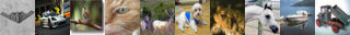
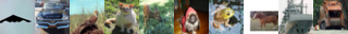
We hypothesize that this variability is caused by the quality of the labeled examples in a given dataset and that selecting low-quality examples might make it more difficult for the model to learn some particular class effectively. To test this, we construct eight new training datasets with examples ranging in “prototypicality” (i.e., representative of the underlying class). Specifically, we take the ordering of the CIFAR-10 training set from [4] that sorts examples from those that are most representative to those that are least. This example ordering was determined after training many CIFAR-10 models with all labeled data. We thus do not envision this as a practical method for actually choosing examples for use in SSL, but rather to experimentally verify that examples that are more representative are better suited for low-label training. We divide this ordering evenly into eight buckets (so all of the most representative examples are in the first bucket, and all of the outliers in the last). We then create eight labeled training sets by randomly selecting one labeled example of each class from the same bucket.
Using the same hyperparameters, the model trained only on the most prototypical examples reaches a median of 78% accuracy (with a maximum of 84% accuracy); training on the middle of the distribution reaches 65% accuracy; and training on only the outliers fails to converge completely, with 10% accuracy. Figure 2 shows the full labeled training dataset for the split where FixMatch achieved a median accuracy of 78%. Further analysis is presented in Appendix B.3.

| Ablation | FixMatch | Only CutOut | No CutOut |
| Error | 4.84 | 6.15 | 6.15 |
5 . Ablation Study
Since FixMatch comprises a simple combination of two existing techniques, we perform an extensive ablation study to better understand why it is able to obtain state-of-the-art results. Recall that we report the mean and the standard deviation over 5 folds for each experimental protocol as our main results in table 2 and table 3. Due to the number of experiments in our ablation study, however, we focus on studying with a single 250 label split from CIFAR-10 and only report results using CTAugment. Note that FixMatch with default parameters achieves 4.84% error rate on this particular split. We present complete results in the supplementary material.
5.1 . Sharpening and Thresholding
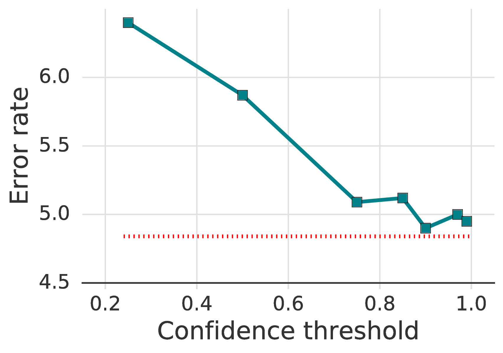
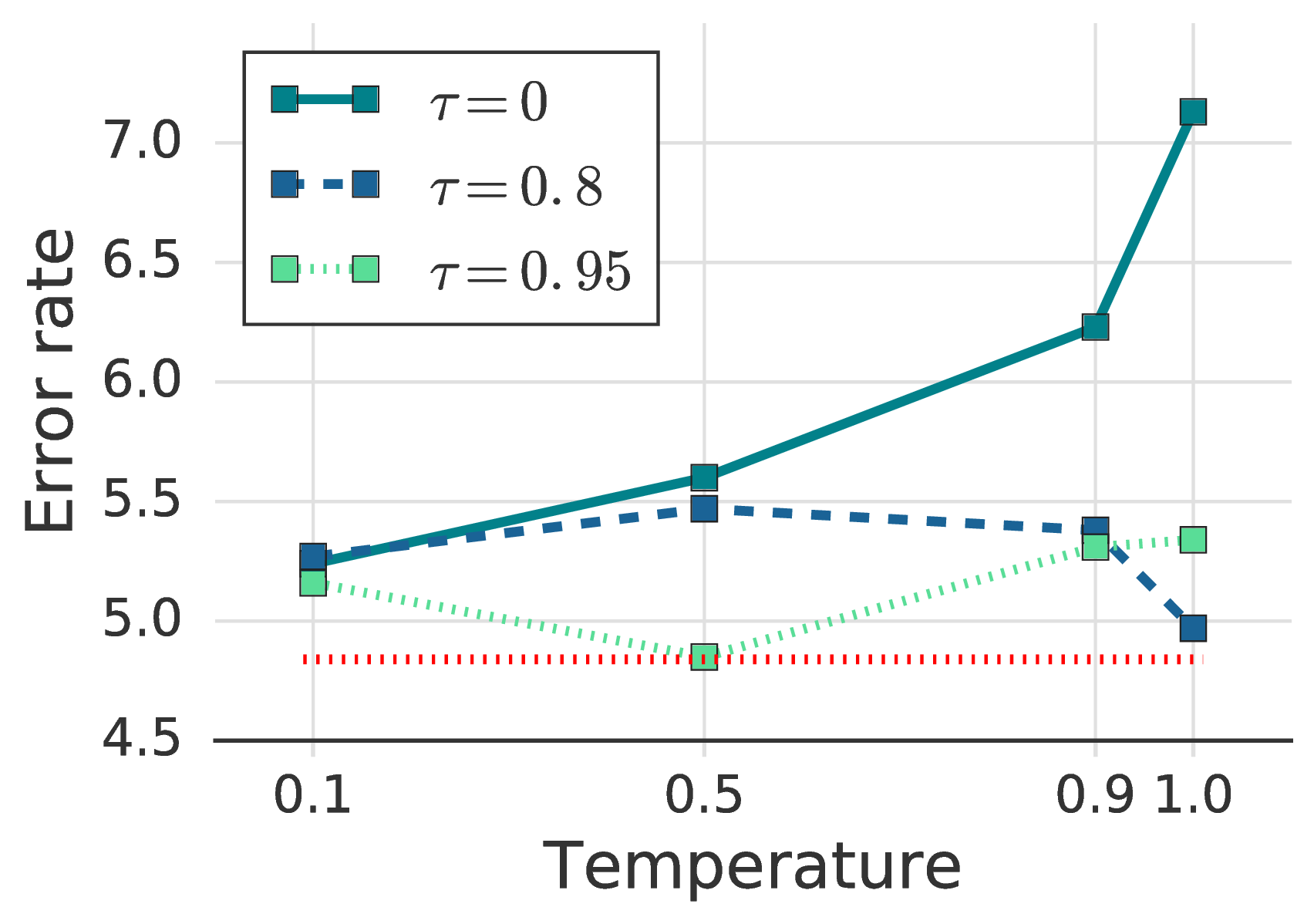
A “soft” version of pseudo-labeling can be designed by sharpening the predicted distribution instead of using one-hot labels. This formulation appears in UDA and is of general interest since other methods such as MixMatch and ReMixMatch also make use of sharpening (albeit without thresholding). Using sharpening instead of an argmax introduces a hyper-parameter: the temperature T [2, 45].
We study the interactions between the temperature T and the confidence threshold τ. Note that pseudo-labeling in FixMatch is recovered as T → 0. The results are presented in fig. 3b and fig. 3c. The threshold value of 0.95 shows the lowest error rate, though increasing it to 0.97 or 0.99 did not hurt the performance. On the other hand, accuracy drops by more than 1.5% when using a small threshold value. Sharpening, on the other hand, did not show a significant difference in performance when a confidence threshold is used. In summary, we observe that swapping pseudo-labeling for sharpening and thresholding would introduce a new hyperparameter while achieving no better performance.
5.2 . Augmentation Strategy
We conduct an ablation study on different strong data augmentation policies as data augmentation plays a key role in FixMatch. Specifically, we chose RandAugment [10] and CTAugment [2], which have been used for state-of-the-art SSL algorithms such as UDA [45] and ReMixMatch [3] respectively. On CIFAR-10, CIFAR-100, and SVHN we observed highly comparable results between the two policies (table 2), whereas in table 3, we observe a significant gain by using CTAugment.
As mentioned in 2.3, CutOut [13] is used by default after strong augmentation in both RandAugment and CTAugment. We therefore measure the effect of CutOut in table 7. We find that both CutOut and CTAugment are required to obtain the best performance; removing either results in a comparable increase in error rate.
We also study different combinations of weak and strong augmentations for pseudo-label generation and prediction (i.e., the upper and lower paths in fig. 1). When we replaced the weak augmentation for label guessing with strong augmentation, we found that the model diverged early in training. This suggests that the pseudo-label needs to be generated using weakly augmented data. Using weak augmentation in place of strong augmentation to generate the model’s prediction for training peaked at 45% accuracy but was not stable and progressively collapsed to 12%, suggesting the importance of strong data augmentation for model prediction at training. This observation is well-aligned with those from supervised learning [9].
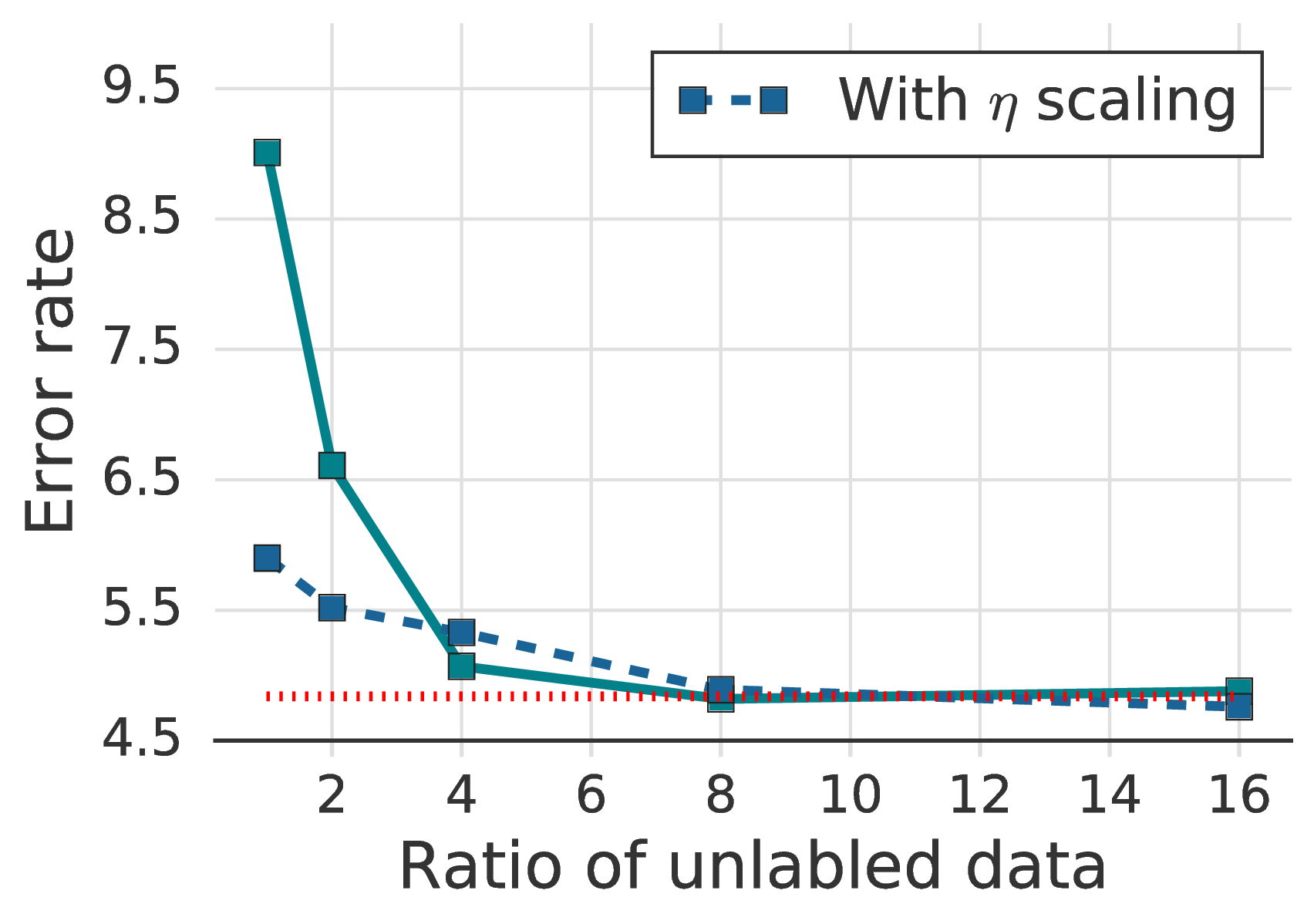
5.3 . Ratio of Unlabeled Data
In fig. 3a we plot the error rates of FixMatch with different ratios of unlabeled data (μ). We observe a significant decrease in error rates by using a large amount of unlabeled data, which is consistent with the finding in UDA [45]. In addition, scaling the learning rate η linearly with the batch size (a technique for large-batch supervised training [15]) was effective for FixMatch, especially when μ is small.
5.4 . Optimizer and Learning Rate Schedule
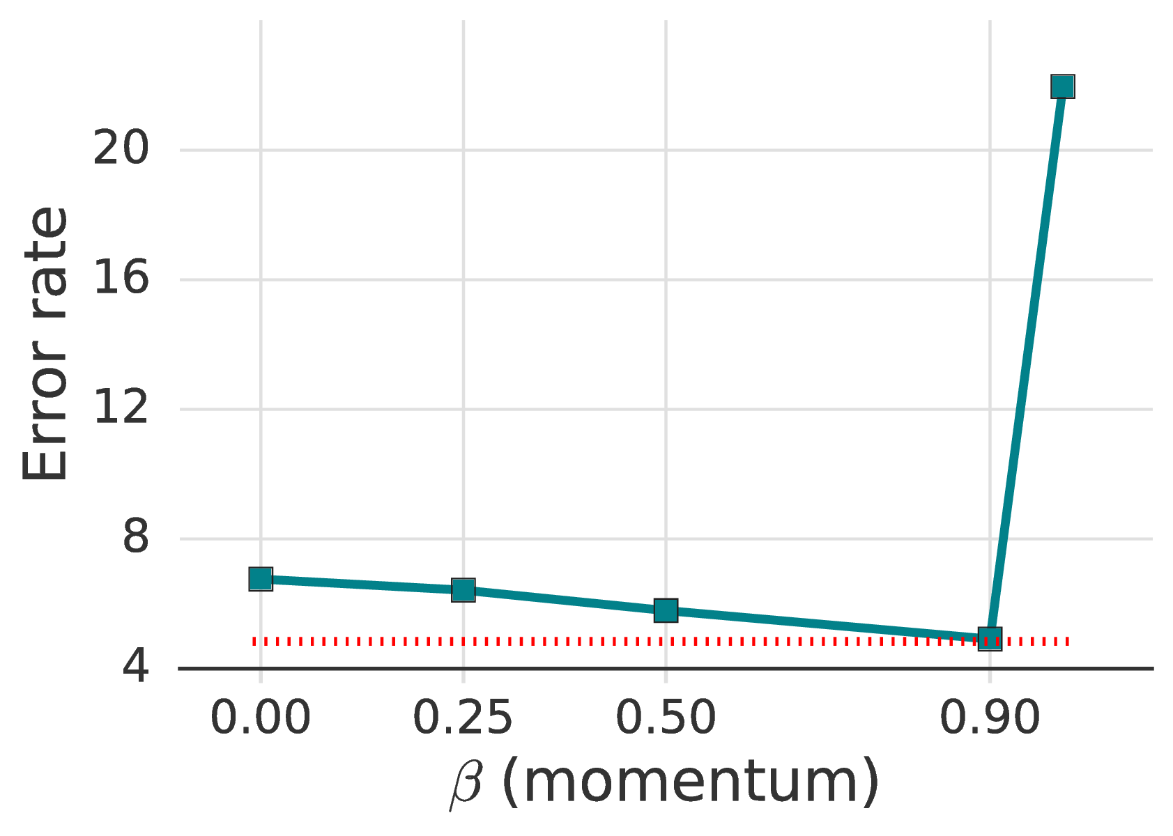
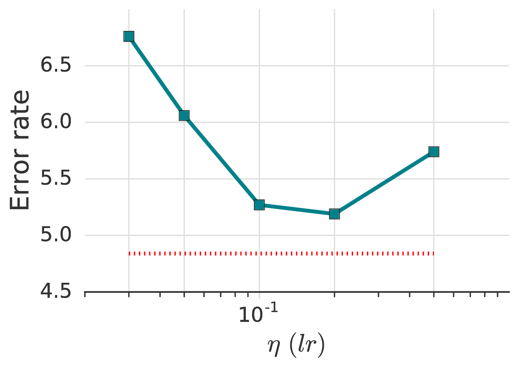
While the study of different optimizers and their hyperparameters is seldom done in previous SSL works, we found that they can have a strong effect on performance. As shown in table 5, SGD with momentum of 0.9 works the best. Without momentum, the best error rate we could reach is 5.19%, compared to 4.84 with momentum. We found that the Nesterov variant of momentum [42] is not required for achieving an error below 5%. For Adam [19], none of the combinations of parameters for η,β1,β2 that we explored appeared competitive with momentum. We refer table 9 in the supplementary material for more details.
It is a popular choice in recent works [23] to use a cosine learning rate decay. In our experiments, a linear learning rate decay performed nearly as well. Note that, as for the cosine learning rate decay, picking a proper decaying rate is important. Finally, using no decay results in worse accuracy (a 0.86% degradation).
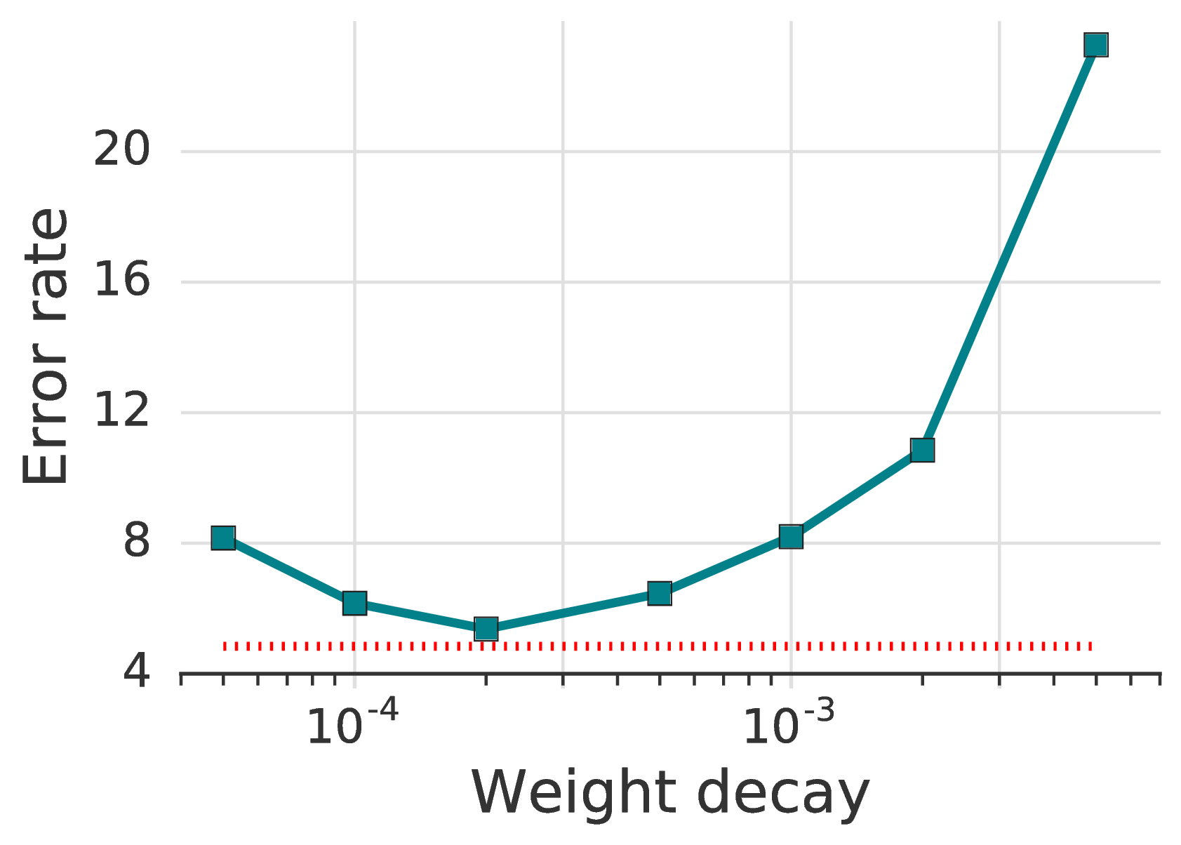
5.5 . Weight Decay
We find that tuning the weight decay is exceptionally important for low-label regimes: choosing a value that is just one order of magnitude larger or smaller than optimal can cost ten percentage points or more, as shown in fig. 3d.
6 . Conclusion
There has been rapid recent progress in semi-supervised learning. Unfortunately, much of this progress comes at the cost of increasingly complicated learning algorithms with sophisticated loss terms and numerous difficult-to-tune hyper-parameters. We introduce FixMatch, a simpler semi-supervised learning algorithm that achieves state-of-the-art results across many datasets. We also show how FixMatch can begin to bridge the gap between low-label semi-supervised learning and few-shot learning—or even clustering: we obtain surprisingly-high accuracy with just one label per class. Using only standard cross-entropy losses on both labeled and unlabeled data, FixMatch’s training objective can be written in just a few lines of code.
Because of this simplicity, we are able to investigate nearly all aspects of the algorithm to understand why it works. We find that to obtain strong results, especially in the limited-label regime, certain design choices are often underemphasized – most importantly, weight decay and the choice of optimizer. The importance of these factors means that even when controlling for model architecture as is recommended in [31], the same technique can not always be directly compared across different implementations.
On the whole, we believe that the existence of such simple but performant semi-supervised machine learning algorithms will help to allow machine learning to be deployed in increasingly many practical domains where labels are expensive or difficult to obtain.
Acknowledgment We thank Qizhe Xie, Avital Oliver and Sercan Arik for their feedback on this paper.
References
[1] Eric Arazo, Diego Ortego, Paul Albert, Noel E. O’Connor, and Kevin McGuinness. Pseudo-labeling and confirmation bias in deep semi-supervised learning. arXiv preprint arXiv:1908.02983, 2019.
[2] David Berthelot, Nicholas Carlini, Ekin D. Cubuk, Alex Kurakin, Kihyuk Sohn, Han Zhang, and Colin Raffel. Remixmatch: Semi-supervised learning with distribution matching and augmentation anchoring. In Eighth International Conference on Learning Representations, 2020.
[3] David Berthelot, Nicholas Carlini, Ian Goodfellow, Nicolas Papernot, Avital Oliver, and Colin A Raffel. Mixmatch: A holistic approach to semi-supervised learning. In Advances in Neural Information Processing Systems 32. 2019.
[4] Nicholas Carlini, Úlfar Erlingsson, and Nicolas Papernot. Distribution density, tails, and outliers in machine learning: Metrics and applications. arXiv preprint arXiv:1910.13427, 2019.
[5] Olivier Chapelle, Bernhard Scholkopf, and Alexander Zien. Semi-Supervised Learning. MIT Press, 2006.
[6] Jinghui Chen and Quanquan Gu. Closing the generalization gap of adaptive gradient methods in training deep neural networks. arXiv preprint arXiv:1806.06763, 2018.
[7] Dami Choi, Christopher J Shallue, Zachary Nado, Jaehoon Lee, Chris J Maddison, and George E Dahl. On empirical comparisons of optimizers for deep learning. arXiv preprint arXiv:1910.05446, 2019.
[8] Adam Coates, Andrew Ng, and Honglak Lee. An analysis of single-layer networks in unsupervised feature learning. In Proceedings of the Fourteenth International Conference on Artificial Intelligence and Statistics, 2011.
[9] Ekin D. Cubuk, Barret Zoph, Dandelion Mane, Vijay Vasudevan, and Quoc V. Le. Autoaugment: Learning augmentation strategies from data. In The IEEE Conference on Computer Vision and Pattern Recognition (CVPR), June 2019.
[10] Ekin D. Cubuk, Barret Zoph, Jonathon Shlens, and Quoc V. Le. Randaugment: Practical automated data augmentation with a reduced search space. arXiv preprint arXiv:1909.13719, 2019.
[11] Zihang Dai, Zhilin Yang, Fan Yang, William W. Cohen, and Ruslan R. Salakhutdinov. Good semi-supervised learning that requires a bad GAN. In Advances in Neural Information Processing Systems, 2017.
[12] Jia Deng, Wei Dong, Richard Socher, Li-Jia Li, Kai Li, and Li Fei-Fei. ImageNet: A large-scale hierarchical image database. In IEEE Conference on Computer Vision and Pattern Recognition, 2009.
[13] Terrance DeVries and Graham W Taylor. Improved regularization of convolutional neural networks with cutout. arXiv preprint arXiv:1708.04552, 2017.
[14] Geoffrey French, Michal Mackiewicz, and Mark Fisher. Self-ensembling for visual domain adaptation. In Sixth International Conference on Learning Representations, 2018.
[15] Priya Goyal, Piotr Dollár, Ross Girshick, Pieter Noordhuis, Lukasz Wesolowski, Aapo Kyrola, Andrew Tulloch, Yangqing Jia, and Kaiming He. Accurate, large minibatch sgd: Training imagenet in 1 hour. arXiv preprint arXiv:1706.02677, 2017.
[16] Yves Grandvalet and Yoshua Bengio. Semi-supervised learning by entropy minimization. In Advances in neural information processing systems, 2005.
[17] Joel Hestness, Sharan Narang, Newsha Ardalani, Gregory Diamos, Heewoo Jun, Hassan Kianinejad, Md. Mostofa Ali Patwary, Yang Yang, and Yanqi Zhou. Deep learning scaling is predictable, empirically. arXiv preprint arXiv:1712.00409, 2017.
[18] Rafal Jozefowicz, Oriol Vinyals, Mike Schuster, Noam Shazeer, and Yonghui Wu. Exploring the limits of language modeling. arXiv preprint arXiv:1602.02410, 2016.
[19] Diederik P Kingma and Jimmy Ba. Adam: A method for stochastic optimization. In Third International Conference on Learning Representations, 2015.
[20] Alex Krizhevsky. Learning multiple layers of features from tiny images. Technical report, University of Toronto, 2009.
[21] Samuli Laine and Timo Aila. Temporal ensembling for semi-supervised learning. In Fifth International Conference on Learning Representations, 2017.
[22] Dong-Hyun Lee. Pseudo-label: The simple and efficient semi-supervised learning method for deep neural networks. In ICML Workshop on Challenges in Representation Learning, 2013.
[23] Ilya Loshchilov and Frank Hutter. SGDR: Stochastic gradient descent with warm restarts. In Fifth International Conference on Learning Representations, 2017.
[24] Ilya Loshchilov and Frank Hutter. Decoupled weight decay regularization. In Sixth International Conference on Learning Representations, 2018.
[25] Dhruv Mahajan, Ross Girshick, Vignesh Ramanathan, Kaiming He, Manohar Paluri, Yixuan Li, Ashwin Bharambe, and Laurens van der Maaten. Exploring the limits of weakly supervised pretraining. In Proceedings of the European Conference on Computer Vision (ECCV), 2018.
[26] David McClosky, Eugene Charniak, and Mark Johnson. Effective self-training for parsing. In Proceedings of the main conference on human language technology conference of the North American Chapter of the Association of Computational Linguistics. Association for Computational Linguistics, 2006.
[27] Geoffrey J. McLachlan. Iterative reclassification procedure for constructing an asymptotically optimal rule of allocation in discriminant analysis. Journal of the American Statistical Association, 70(350):365–369, 1975.
[28] Takeru Miyato, Shin-ichi Maeda, Shin Ishii, and Masanori Koyama. Virtual adversarial training: a regularization method for supervised and semi-supervised learning. IEEE transactions on pattern analysis and machine intelligence, 2018.
[29] Yurii Evgen’evich Nesterov. A method of solving a convex programming problem with convergence rate o(k̂2). Doklady Akademii Nauk, 269(3), 1983.
[30] Yuval Netzer, Tao Wang, Adam Coates, Alessandro Bissacco, Bo Wu, and Andrew Y. Ng. Reading digits in natural images with unsupervised feature learning. In NIPS Workshop on Deep Learning and Unsupervised Feature Learning, 2011.
[31] Avital Oliver, Augustus Odena, Colin A Raffel, Ekin Dogus Cubuk, and Ian Goodfellow. Realistic evaluation of deep semi-supervised learning algorithms. In Advances in Neural Information Processing Systems, pages 3235–3246, 2018.
[32] Hieu Pham and Quoc V Le. Semi-supervised learning by coaching. Submitted to the 8th International Conference on Learning Representations, 2019. https://openreview.net/forum?id=rJe04p4YDB.
[33] Boris T Polyak. Some methods of speeding up the convergence of iteration methods. USSR Computational Mathematics and Mathematical Physics, 4(5), 1964.
[34] Alec Radford, Jeffrey Wu, Rewon Child, David Luan, Dario Amodei, and Ilya Sutskever. Language models are unsupervised multitask learners, 2019.
[35] Colin Raffel, Noam Shazeer, Adam Roberts, Katherine Lee, Sharan Narang, Michael Matena, Yanqi Zhou, Wei Li, and Peter J. Liu. Exploring the limits of transfer learning with a unified text-to-text transformer. arXiv preprint arXiv:1910.10683, 2019.
[36] Antti Rasmus, Mathias Berglund, Mikko Honkala, Harri Valpola, and Tapani Raiko. Semi-supervised learning with ladder networks. In Advances in Neural Information Processing Systems, 2015.
[37] Chuck Rosenberg, Martial Hebert, and Henry Schneiderman. Semi-supervised self-training of object detection models. In Proceedings of the Seventh IEEE Workshops on Application of Computer Vision, 2005.
[38] Mehdi Sajjadi, Mehran Javanmardi, and Tolga Tasdizen. Mutual exclusivity loss for semi-supervised deep learning. In IEEE International Conference on Image Processing, 2016.
[39] Mehdi Sajjadi, Mehran Javanmardi, and Tolga Tasdizen. Regularization with stochastic transformations and perturbations for deep semi-supervised learning. In Advances in Neural Information Processing Systems, 2016.
[40] H Scudder. Probability of error of some adaptive pattern-recognition machines. IEEE Transactions on Information Theory, 11(3), 1965.
[41] Nitish Srivastava, Geoffrey Hinton, Alex Krizhevsky, Ilya Sutskever, and Ruslan Salakhutdinov. Dropout: a simple way to prevent neural networks from overfitting. The journal of machine learning research, 15(1), 2014.
[42] Ilya Sutskever, James Martens, George Dahl, and Geoffrey Hinton. On the importance of initialization and momentum in deep learning. In International conference on machine learning, 2013.
[43] Antti Tarvainen and Harri Valpola. Mean teachers are better role models: Weight-averaged consistency targets improve semi-supervised deep learning results. In Advances in neural information processing systems, 2017.
[44] Ashia C Wilson, Rebecca Roelofs, Mitchell Stern, Nati Srebro, and Benjamin Recht. The marginal value of adaptive gradient methods in machine learning. In Advances in Neural Information Processing Systems, pages 4148–4158, 2017.
[45] Qizhe Xie, Zihang Dai, Eduard Hovy, Minh-Thang Luong, and Quoc V. Le. Unsupervised data augmentation for consistency training. arXiv preprint arXiv:1904.12848, 2019.
[46] Qizhe Xie, Eduard Hovy, Minh-Thang Luong, and Quoc V. Le. Self-training with noisy student improves ImageNet classification. arXiv preprint arXiv:1911.04252, 2019.
[47] Sergey Zagoruyko and Nikos Komodakis. Wide residual networks. In Proceedings of the British Machine Vision Conference (BMVC), 2016.
[48] Xiaohua Zhai, Avital Oliver, Alexander Kolesnikov, and Lucas Beyer. S4l: Self-supervised semi-supervised learning. In The IEEE International Conference on Computer Vision (ICCV), October 2019.
[49] Guodong Zhang, Chaoqi Wang, Bowen Xu, and Roger Grosse. Three mechanisms of weight decay regularization. arXiv preprint arXiv:1810.12281, 2018.
[50] Hongyi Zhang, Moustapha Cisse, Yann N. Dauphin, and David Lopez-Paz. MixUp: Beyond empirical risk minimization. arXiv preprint arXiv:1710.09412, 2017.
[51] Xiaojin Zhu. Semi-supervised learning literature survey. Technical Report TR 1530, Computer Sciences, University of Wisconsin – Madison, 2008.
[52] Xiaojin Zhu and Andrew B Goldberg. Introduction to semi-supervised learning. Synthesis lectures on artificial intelligence and machine learning, 3(1), 2009.
[53] Yang Zou, Zhiding Yu, BVK Vijaya Kumar, and Jinsong Wang. Unsupervised domain adaptation for semantic segmentation via class-balanced self-training. In Proceedings of the European Conference on Computer Vision (ECCV), pages 289–305, 2018.
A . Algorithm
We present the complete algorithm for FixMatch in algorithm 1.

B . Comprehensive Experimental Results
B.1 . Hyperparameters
As mentioned in section 4, we used almost identical hyperparameters of FixMatch on CIFAR-10, CIFAR-100, SVHN and STL-10. Note that we used similar network architectures for these datasets, except that more convolution filters were used for CIFAR-100 to handle larger label space and more convolutions were used for STL-10 to deal with larger input image size. Here, we provide a complete list of hyperparameters in table 8. Note that we did ablation study for most of these hyperparameters in section 5 (τ in section 5.1, μ in section 5.3, lr and β (momentum) in section 5.4, and weight decay in section 5.5).
B.2 . Full Ablation Results on Optimizers
We present full ablation results on optimizers in table 9. First, we studied the effect of momentum (β) for SGD optimizer. We found that the performance is somewhat sensitive to β and the model did not converge when β is set too large. On the other hand, small values of β still worked fine. When β is small, increasing the learning rate improved the performance, though they are not as good as the best performance obtained with β=0.9. Nesterov momentum resulted in a slightly lower error rate than that of standard momentum SGD, but the difference was not significant.
As studied in [44, 24], we did not find Adam performing better than momentum SGD. While the best error rate of the model trained with Adam is only 0.53% larger than that of momentum SGD, we found that the performance was much more sensitive to the change of learning rate (e.g., increase in error rate by more than 8% when increasing the learning rate to 0.002) than momentum SGD. Additional exploration along this direction to make Adam more competitive includes the use of weight decay [24, 49] instead of L2 weight regularization and a better exploration of hyperparameters [6, 7].
| Optimizer | Hyperparameters | Error | ||
| SGD | η = 0.03 | β = 0.90 | Nesterov | 4.84 |
| SGD | η = 0.03 | β = 0.999 | Nesterov | 84.33 |
| SGD | η = 0.03 | β = 0.99 | Nesterov | 21.97 |
| SGD | η = 0.03 | β = 0.50 | Nesterov | 5.79 |
| SGD | η = 0.03 | β = 0.25 | Nesterov | 6.42 |
| SGD | η = 0.03 | β = 0 | Nesterov | 6.76 |
| SGD | η = 0.05 | β = 0 | Nesterov | 6.06 |
| SGD | η = 0.10 | β = 0 | Nesterov | 5.27 |
| SGD | η = 0.20 | β = 0 | Nesterov | 5.19 |
| SGD | η = 0.50 | β = 0 | Nesterov | 5.74 |
| SGD | η = 0.03 | β = 0.90 | 4.86 | |
| Adam | η = 0.002 | β1 = 0.9 | β2 = 0.00 | 29.42 |
| Adam | η = 0.002 | β1 = 0.9 | β2 = 0.90 | 14.42 |
| Adam | η = 0.002 | β1 = 0.9 | β2 = 0.99 | 15.44 |
| Adam | η = 0.002 | β1 = 0.9 | β2 = 0.999 | 13.93 |
| Adam | η = 0.0008 | β1 = 0.9 | β2 = 0.999 | 7.35 |
| Adam | η = 0.0006 | β1 = 0.9 | β2 = 0.999 | 6.12 |
| Adam | η = 0.0005 | β1 = 0.9 | β2 = 0.999 | 5.95 |
| Adam | η = 0.0004 | β1 = 0.9 | β2 = 0.999 | 5.44 |
| Adam | η = 0.0003 | β1 = 0.9 | β2 = 0.999 | 5.37 |
| Adam | η = 0.0002 | β1 = 0.9 | β2 = 0.999 | 5.57 |
| Adam | η = 0.0001 | β1 = 0.9 | β2 = 0.999 | 7.90 |
B.3 . Labeled Data for Barely Supervised Learning
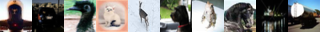
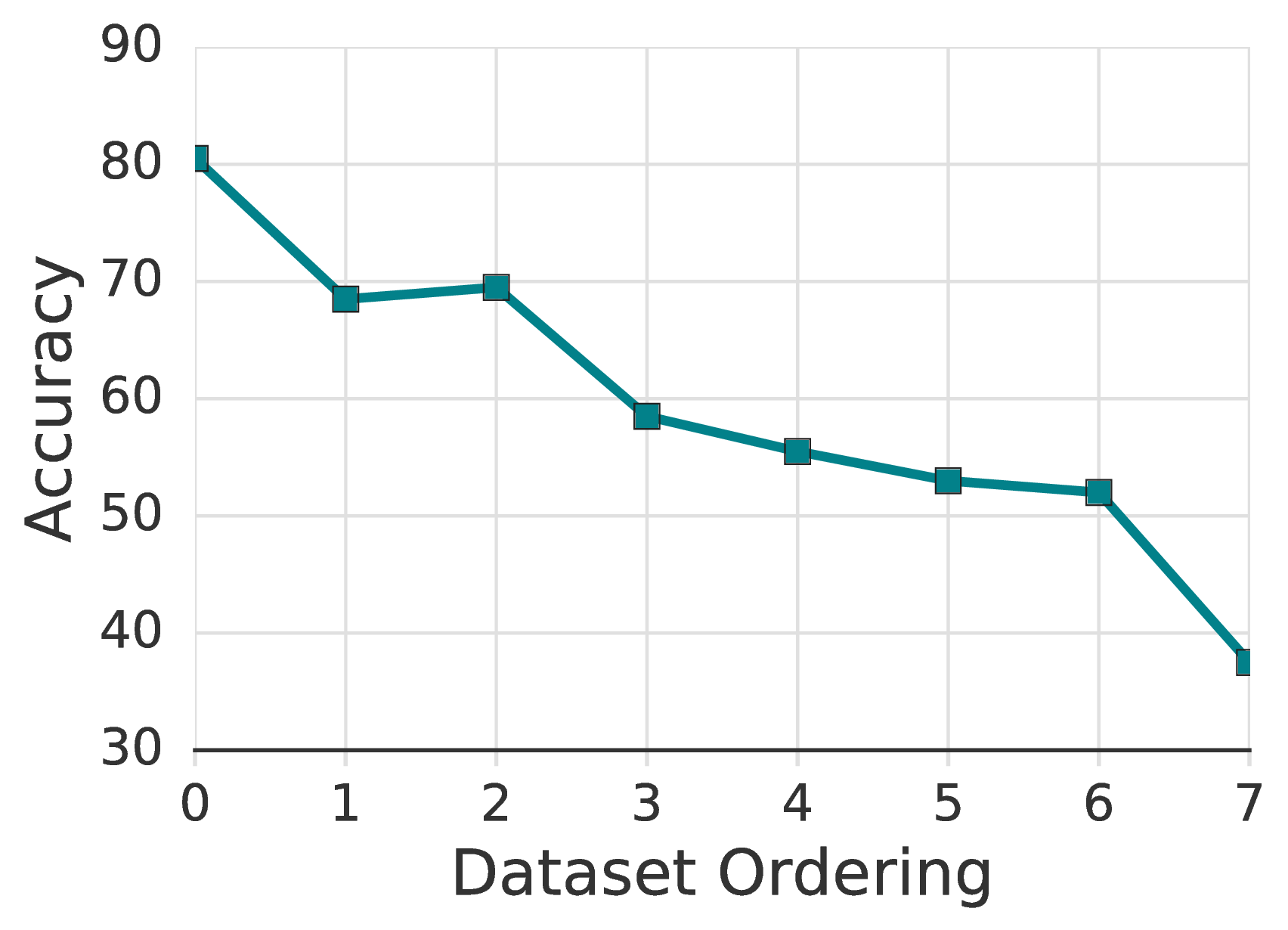
In addition to fig. 2, we visualize the full labeled training images obtained by ordering mechanism [4] used for barely supervised learning in fig. 5. Each row contains 10 images from 10 different classes of CIFAR-10 and is used as the complete labeled training dataset for one run of FixMatch. The first row contains the most prototypical images of each class, while the bottom row contains the least prototypical images. We train two models for each dataset and compute the mean accuracy between the two and plot this in fig. 6. Observe that we obtain over 80% accuracy when training on the best examples.


B.4 . Comparison to Supervised Baselines
In table 10 and table 11, we present the performance of models trained only with the labeled data using strong data augmentations to highlight the effectiveness of using unlabeled data in FixMatch.
| CIFAR-10 | CIFAR-100 | SVHN
| |||||||
| Method | 40 labels | 250 labels | 4000 labels | 400 labels | 2500 labels | 10000 labels | 40 labels | 250 labels | 1000 labels |
| Supervised (RA) | 64.01±0.76 | 39.12±0.77 | 12.74±0.29 | 79.47±0.18 | 52.88±0.51 | 32.55±0.21 | 52.68±2.29 | 22.48±0.55 | 10.89±0.12 |
| Supervised (CTA) | 64.53±0.83 | 41.92±1.17 | 13.64±0.12 | 79.79±0.59 | 54.23±0.48 | 35.30±0.19 | 43.05±2.34 | 15.06±1.02 | 7.69±0.27 |
| FixMatch (RA) | 13.81±3.37 | 5.07±0.65 | 4.26±0.05 | 48.85±1.75 | 28.29±0.11 | 22.60±0.12 | 3.96±2.17 | 2.48±0.38 | 2.28±0.11 |
| FixMatch (CTA) | 11.39±3.35 | 5.07±0.33 | 4.31±0.15 | 49.95±3.01 | 28.64±0.24 | 23.18±0.11 | 7.65±7.65 | 2.64±0.64 | 2.36±0.19 |
C . Implementation Details for Section 4.3
For our ImageNet experiments we use standard ResNet50 pre-activation model trained in a distributed way on a TPU device with 32 cores.4 We report results over five random folds of labeled data. We use following set of hyperparameters for our ImageNet model:
- Batch size. On each step our batch contains 1024 labeled examples and 5120 unlabeled examples.
- Training time. We train our model for 300 epochs of unlabeled examples.
- Learning rate schedule. We utilize linear learning rate warmup for the first 5 epochs until it reaches an initial value of 0.4. Then we the decay learning rate at epochs 60, 120, 160, and 200 epoch by multiplying it by 0.1.
- Optimizer. We use Nesterov Momentum optimizer with momentum 0.9.
- Exponential moving average (EMA). We utilize EMA technique with decay 0.999.
- FixMatch loss. We use unlabeled loss weight λu = 10 and confidence threshold τ = 0.7 in FixMatch loss.
- Weight decay. Our weight decay coefficient is 0.0001. Similarly to other datasets we perform weight decay by adding L2 penalty of all weights to model loss.
- Augmentation of unlabeled images. For strong augmentation we use RandAugment with random magnitude [10]. For weak augmentation we use a random horizontal flip.
- ImageNet preprocessing. We randomly crop and rescale to 224×224 size all labeled and unlabeled training images prior to performing augmentation. This is considered a standard ImageNet preprocessing technique.
D . List of Data Transformations
We used the same sets of image transformations used in RandAugment [10] and CTAugment [2]. For completeness, we listed all transformation operations for these augmentation strategies in table 12 and table 13.
| Transformation | Description | Parameter | Range |
| Autocontrast | Maximizes the image contrast by setting the darkest (lightest) pixel to black (white). |
|
|
| Brightness | Adjusts the brightness of the image. B = 0 returns a black image, B = 1 returns the original image. | B | [0.05, 0.95] |
| Color | Adjusts the color balance of the image like in a TV. C = 0 returns a black & white image, C = 1 returns the original image. | C | [0.05, 0.95] |
| Contrast | Controls the contrast of the image. A C = 0 returns a gray image, C = 1 returns the original image. | C | [0.05, 0.95] |
| Equalize | Equalizes the image histogram. |
|
|
| Identity | Returns the original image. |
|
|
| Posterize | Reduces each pixel to B bits. | B | [4, 8] |
| Rotate | Rotates the image by θ degrees. | θ | [-30, 30] |
| Sharpness | Adjusts the sharpness of the image, where S = 0 returns a blurred image, and S = 1 returns the original image. | S | [0.05, 0.95] |
| Shear_x | Shears the image along the horizontal axis with rate R. | R | [-0.3, 0.3] |
| Shear_y | Shears the image along the vertical axis with rate R. | R | [-0.3, 0.3] |
| Solarize | Inverts all pixels above a threshold value of T. | T | [0, 1] |
| Translate_x | Translates the image horizontally by (λ×image width) pixels. | λ | [-0.3, 0.3] |
| Translate_y | Translates the image vertically by (λ×image height) pixels. | λ | [-0.3, 0.3] |
| Transformation | Description | Parameter | Range |
| Autocontrast | Maximizes the image contrast by setting the darkest (lightest) pixel to black (white), and then blends with the original image with blending ratio λ. | λ | [0, 1] |
| Brightness | Adjusts the brightness of the image. B = 0 returns a black image, B = 1 returns the original image. | B | [0, 1] |
| Color | Adjusts the color balance of the image like in a TV. C = 0 returns a black & white image, C = 1 returns the original image. | C | [0, 1] |
| Contrast | Controls the contrast of the image. A C = 0 returns a gray image, C = 1 returns the original image. | C | [0, 1] |
| Cutout | Sets a random square patch of side-length (L×image width) pixels to gray. | L | [0, 0.5] |
| Equalize | Equalizes the image histogram, and then blends with the original image with blending ratio λ. | λ | [0, 1] |
| Invert | Inverts the pixels of the image, and then blends with the original image with blending ratio λ. | λ | [0, 1] |
| Identity | Returns the original image. |
|
|
| Posterize | Reduces each pixel to B bits. | B | [1, 8] |
| Rescale | Takes a center crop that is of side-length (L×image width), and rescales to the original image size using method M. | L | [0.5, 1.0] |
|
| M | see caption |
|
| Rotate | Rotates the image by θ degrees. | θ | [-45, 45] |
| Sharpness | Adjusts the sharpness of the image, where S = 0 returns a blurred image, and S = 1 returns the original image. | S | [0, 1] |
| Shear_x | Shears the image along the horizontal axis with rate R. | R | [-0.3, 0.3] |
| Shear_y | Shears the image along the vertical axis with rate R. | R | [-0.3, 0.3] |
| Smooth | Adjusts the smoothness of the image, where S = 0 returns a maximally smooth image, and S = 1 returns the original image. | S | [0, 1] |
| Solarize | Inverts all pixels above a threshold value of T. | T | [0, 1] |
| Translate_x | Translates the image horizontally by (λ×image width) pixels. | λ | [-0.3, 0.3] |
| Translate_y | Translates the image vertically by (λ×image height) pixels. | λ | [-0.3, 0.3] |