Fine-Tuning Pre-trained Language Model with Weak Supervision:
A Contrastive-Regularized Self-Training Approach

Abstract

Fine-tuned pre-trained language models (LMs) have achieved enormous success in many natural language processing (NLP) tasks, but they still require excessive labeled data in the fine-tuning stage. We study the problem of fine-tuning pre-trained LMs using only weak supervision, without any labeled data. This problem is challenging because the high capacity of LMs makes them prone to overfitting the noisy labels generated by weak supervision. To address this problem, we develop a contrastive self-training framework, COSINE, to enable fine-tuning LMs with weak supervision. Underpinned by contrastive regularization and confidence-based reweighting, our framework gradually improves model fitting while effectively suppressing error propagation. Experiments on sequence, token, and sentence pair classification tasks show that our model outperforms the strongest baseline by large margins and achieves competitive performance with fully-supervised fine-tuning methods. Our implementation is available on https://github.com/yueyu1030/COSINE.

1 Introduction

Language model (LM) pre-training and fine-tuning achieve state-of-the-art performance in various natural language processing tasks Peters et al. (2018); Devlin et al. (2019); Liu et al. (2019); Raffel et al. (2019). Such approaches stack task-specific layers on top of pre-trained language models, e.g., BERT Devlin et al. (2019), then fine-tune the models with task-specific data. During fine-tuning, the semantic and syntactic knowledge in the pre-trained LMs is adapted for the target task. Despite their success, one bottleneck for fine-tuning LMs is the requirement of labeled data. When labeled data are scarce, the fine-tuned models often suffer from degraded performance, and the large number of parameters can cause severe overfitting Xie et al. (2019).

To relieve the label scarcity bottleneck, we fine-tune the pre-trained language models with only weak supervision. While collecting large amounts of clean labeled data is expensive for many NLP tasks, it is often cheap to obtain weakly labeled data from various weak supervision sources, such as semantic rules Awasthi et al. (2020). For example, in sentiment analysis, we can use rules ‘terrible’$\mathrm{\to }$Negative (a keyword rule) and ‘* not recommend *’$\mathrm{\to }$Negative (a pattern rule) to generate large amounts of weak labels.

Fine-tuning language models with weak supervision is nontrivial. Excessive label noise, e.g., wrong labels, and limited label coverage are common and inevitable in weak supervision. Although existing fine-tuning approaches Xu et al. (2020); Zhu et al. (2020); Jiang et al. (2020) improve LMs’ generalization ability, they are not designed for noisy data and are still easy to overfit on the noise. Moreover, existing works on tackling label noise are flawed and are not designed for fine-tuning LMs. For example, Ratner et al. (2020); Varma and Ré (2018) use probabilistic models to aggregate multiple weak supervisions for denoising, but they generate weak-labels in a context-free manner, without using LMs to encode contextual information of the training samples Aina et al. (2019). Other works Luo et al. (2017); Wang et al. (2019b) focus on noise transitions without explicitly conducting instance-level denoising, and they require clean training samples. Although some recent studies Awasthi et al. (2020); Ren et al. (2020) design labeling function-guided neural modules to denoise each sample, they require prior knowledge on weak supervision, which is often infeasible in real practice.

Self-training Rosenberg et al. (2005); Lee (2013) is a proper tool for fine-tuning language models with weak supervision. It augments the training set with unlabeled data by generating pseudo-labels for them, which improves the models’ generalization power. This resolves the limited coverage issue in weak supervision. However, one major challenge of self-training is that the algorithm still suffers from error propagation—wrong pseudo-labels can cause model performance to gradually deteriorate.

We propose a new algorithm COSINE that fine-tunes pre-trained LMs with only weak supervision. COSINE leverages both weakly labeled and unlabeled data, as well as suppresses label noise via contrastive self-training. Weakly-supervised learning enriches data with potentially noisy labels, and our contrastive self-training scheme fulfills the denoising purpose. Specifically, contrastive self-training regularizes the feature space by pushing samples with the same pseudo-labels close while pulling samples with different pseudo-labels apart. Such regularization enforces representations of samples from different classes to be more distinguishable, such that the classifier can make better decisions. To suppress label noise propagation during contrastive self-training, we propose confidence-based sample reweighting and regularization methods. The reweighting strategy emphasizes samples with high prediction confidence, which are more likely to be correctly classified, in order to reduce the effect of wrong predictions. Confidence regularization encourages smoothness over model predictions, such that no prediction can be over-confident, and therefore reduces the influence of wrong pseudo-labels.

Our model is flexible and can be naturally extended to semi-supervised learning, where a small set of clean labels is available. Moreover, since we do not make assumptions about the nature of the weak labels, COSINE can handle various types of label noise, including biased labels and randomly corrupted labels. Biased labels are usually generated by semantic rules, whereas corrupted labels are often produced by crowd-sourcing.

Our main contributions are: (1) A contrastive-regularized self-training framework that fine-tunes pre-trained LMs with only weak supervision. (2) Confidence-based reweighting and regularization techniques that reduce error propagation and prevent over-confident predictions. (3) Extensive experiments on 6 NLP classification tasks using 7 public benchmarks verifying the efficacy of COSINE. We highlight that our model achieves competitive performance in comparison with fully-supervised models on some datasets, e.g., on the Yelp dataset, we obtain a $97.2\%$ (fully-supervised) v.s. $96.0\%$ (ours) accuracy comparison.

Figure 1: The framework of COSINE. We first fine-tune the pre-trained language model on weakly-labeled data with early stopping. Then, we conduct contrastive-regularized self-training to improve model generalization and reduce the label noise. During self-training, we calculate the confidence of the prediction and update the model with high confidence samples to reduce error propagation.

2 Background

In this section, we introduce weak supervision and our problem formulation.

Weak Supervision. Instead of using human-annotated data, we obtain labels from weak supervision sources, including keywords and semantic rules. From weak supervision sources, each of the input samples $x\in ?$ is given a label $y\in ?\cup \{\mathrm{\varnothing }\}$, where $?$ is the label set and $\mathrm{\varnothing }$ denotes the sample is not matched by any rules. For samples that are given multiple labels, e.g., matched by multiple rules, we determine their labels by majority voting.

Problem Formulation. We focus on the weakly-supervised classification problems in natural language processing. We consider three types of tasks: sequence classification, token classification, and sentence pair classification. These tasks have a broad scope of applications in NLP, and some examples can be found in Table 1.

Formally, the weakly-supervised classification problem is defined as the following: Given weakly-labeled samples ${?}_l={\{(x_i,y_i)\}}_{i=1}^L$ and unlabeled samples ${?}_u={\{x_j\}}_{j=1}^U$, we seek to learn a classifier $f(x;\theta ):?\to ?$. Here $?={?}_l\cup {?}_u$ denotes all the samples and $?=\{1,2,\mathrm{\cdots },C\}$ is the label set, where $C$ is the number of classes.

Formulation	Example Task	Input	Output
Sequence Classification	Sentiment Analysis, Topic Classification, Question Classification	$[{𝒙}_1,\mathrm{\dots },{𝒙}_N]$	$y$
Token Classification	Slot Filling, Part-of-speech Tagging, Event Detection	$[x_1,\mathrm{\dots },x_N]$	$[y_1,\mathrm{\dots },y_N]$
Sentence Pair Classification	Word Sense Disambiguation, Textual Entailment, Reading Comprehension	$[{𝒙}_1,{𝒙}_2]$	$y$

Table 1: Comparison of different tasks. For sequence classification, input is a sequence of sentences, and we output a scalar label. For token classification, input is a sequence of tokens, and we output one scalar label for each token. For sentence pair classification, input is a pair of sentences, and we output a scalar label.

3 Method

Our classifier $f=g\circ \text{BERT}$ consists of two parts: BERT is a pre-trained language model that outputs hidden representations of input samples, and $g$ is a task-specific classification head that outputs a $C$-dimensional vector, where each dimension corresponds to the prediction confidence of a specific class. In this paper, we use RoBERTa Liu et al. (2019) as the realization of BERT.

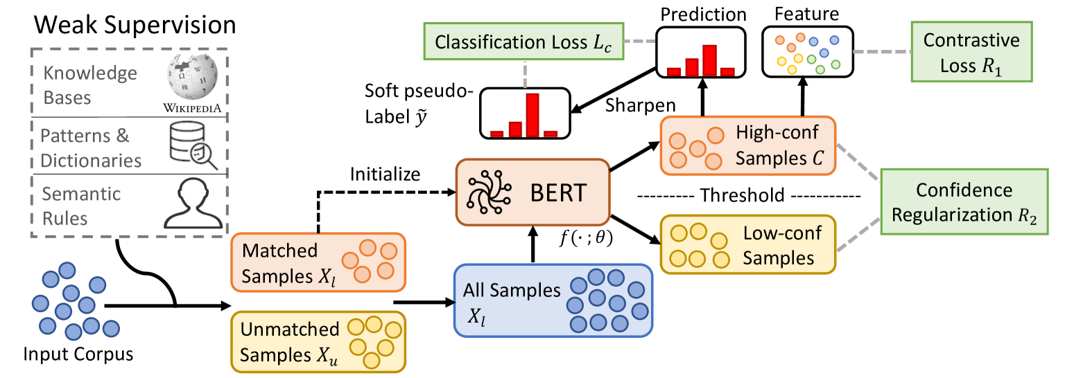
The framework of COSINE is shown in Figure 1. First, COSINE initializes the LM with weak labels. In this step, the semantic and syntactic knowledge of the pre-trained LM are transferred to our model. Then, it uses contrastive self-training to suppress label noise propagation and continue training.

3.1 Overview

The training procedure of COSINE is as follows.

Initialization with Weakly-labeled Data. We fine-tune $f(\cdot ;\theta )$ with weakly-labeled data ${?}_l$ by solving the optimization problem

$$\underset{\theta }{\min }\frac{1}{|{𝒳}_l|}\sum _{(x_i,y_i)\in {𝒳}_l}\text{CE}(f(x_i;\theta ),y_i),$$ (1)

where $\text{CE}(\cdot ,\cdot )$ is the cross entropy loss. We adopt early stopping Dodge et al. (2020) to prevent the model from overfitting to the label noise. However, early stopping causes underfitting, and we resolve this issue by contrastive self-training.

Contrastive Self-training with All Data. The goal of contrastive self-training is to leverage all data, both labeled and unlabeled, for fine-tuning, as well as to reduce the error propagation of wrongly labelled data. We generate pseudo-labels for the unlabeled data and incorporate them into the training set. To reduce error propagation, we introduce contrastive representation learning (Sec. 3.2) and confidence-based sample reweighting and regularization (Sec. 3.3). We update the pseudo-labels (denoted by $\widetilde{?}$) and the model iteratively. The procedures are summarized in Algorithm 1.

$\diamond$ Update $\stackrel{\mathrm{~}}{y}$ with the current $\theta$. To generate the pseudo-label for each sample $x\in ?$, one straight-forward way is to use hard labels Lee (2013)

$${\tilde{y}}_{\text{hard}}=\underset{j\in 𝒴}{\text{argmax}}{\left[f(x;\theta )\right]}_j.$$ (2)

Notice that $f(x;\theta )\in {ℝ}^C$ is a probability vector and ${[f(x;\theta )]}_j$ indicates the $j$-th entry of it. However, these hard pseudo-labels only keep the most likely class for each sample and result in the propagation of labeling mistakes. For example, if a sample is mistakenly classified to a wrong class, assigning a 0/1 label complicates model updating (Eq. 4), in that the model is fitted on erroneous labels. To alleviate this issue, for each sample $x$ in a batch $ℬ$, we generate soft pseudo-labels Xie et al. (2016, 2019); Meng et al. (2020); Liang et al. (2020) $\widetilde{?}\in {ℝ}^C$ based on the current model as

$${\widetilde{𝒚}}_j=\frac{{[f(x;\theta )]}_j^2/f_j}{{\sum }_{j^{\prime }\in 𝒴}{[f(x;\theta )]}_{j^{\prime }}^2/f_{j^{\prime }}},$$ (3)

where $f_j={\sum }_{x^{\prime }\in ℬ}{[f(x^{\prime };\theta )]}_j^2$ is the sum over soft frequencies of class $j$. The non-binary soft pseudo-labels guarantee that, even if our prediction is inaccurate, the error propagated to the model update step will be smaller than using hard pseudo-labels.

$\diamond$ Update $\theta$ with the current $\stackrel{\mathrm{~}}{y}$. We update the model parameters $\theta$ by minimizing

$$ℒ(\theta ;\widetilde{𝒚})={ℒ}_c(\theta ;\widetilde{𝒚})+{ℛ}_1(\theta ;\widetilde{𝒚})+\lambda {ℛ}_2(\theta ),$$ (4)

where ${ℒ}_c$ is the classification loss (Sec. 3.3), ${ℛ}_1(\theta ;\widetilde{?})$ is the contrastive regularizer (Sec. 3.2), ${ℛ}_2(\theta )$ is the confidence regularizer (Sec. 3.3), and $\lambda$ is the hyper-parameter for the regularization.

Input: Training samples $?$; Weakly labeled samples ${?}_l\subseteq ?$; Pre-trained LM $f(\cdot ;\theta )$.

// Fine-tune the LM with weakly-labeled data.

for $t\mathrm{=}\mathrm{1}\mathrm{,}\mathrm{2}\mathrm{,}\mathrm{\cdots }\mathrm{,}{T}_{\mathrm{1}}$ do

       Sample a minibatch $ℬ$ from ${?}_l$.

       Update $\theta$ by Eq. 1 using AdamW.

// Conduct contrastive self-training with all data.

for $t\mathrm{=}\mathrm{1}\mathrm{,}\mathrm{2}\mathrm{,}\mathrm{\cdots }\mathrm{,}{T}_{\mathrm{2}}$ do

       Update pseudo-labels $\widetilde{?}$ by Eq. 3 for all $x\in ?$.

       for $k\mathrm{=}\mathrm{1}\mathrm{,}\mathrm{2}\mathrm{,}\mathrm{\cdots }\mathrm{,}{T}_{\mathrm{3}}$ do

             Sample a minibatch $ℬ$ from $?$.

             Select high confidence samples $?$ by Eq. 9.

             Calculate ${ℒ}_c$ by Eq. 10, ${ℛ}_1$ by Eq. 6, ${ℛ}_2$ by Eq. 12, and $ℒ$ by Eq. 4.

             Update $\theta$ using AdamW.

      

Output: Fine-tuned model $f(\cdot ;\theta )$.

Algorithm 1 Training Procedures of COSINE.

3.2 Contrastive Learning on Sample Pairs

The key ingredient of our contrastive self-training method is to learn representations that encourage data within the same class to have similar representations and keep data in different classes separated. Specifically, we first select high-confidence samples (Sec. 3.3) $?$ from $?$. Then for each pair $x_i,x_j\in ?$, we define their similarity as

(5)

where ${\widetilde{?}}_i$, ${\widetilde{?}}_j$ are the soft pseudo-labels (Eq. 3) for $x_i$, $x_j$, respectively. For each $x\in ?$, we calculate its representation $?=\text{BERT}(x)\in {ℝ}^d$, then we define the contrastive regularizer as

$${ℛ}_1(\theta ;\widetilde{𝒚})=\sum _{(x_i,x_j)\in 𝒞\times 𝒞}\mathrm{\ell }({𝒗}_i,{𝒗}_j,W_{ij}),$$ (6)

where

$$\mathrm{\ell }=W_{ij}{d}_{ij}^2+(1-W_{ij}){[\max (0,\gamma -d_{ij})]}^2.$$ (7)

Here, $\mathrm{\ell }(\cdot ,\cdot ,\cdot )$ is the contrastive loss Chopra et al. (2005); Taigman et al. (2014), $d_{ij}$ is the distance between ${?}_i$ and ${?}_j$, and $\gamma$ is a pre-defined margin.

Figure 2: An illustration of contrastive learning. The black solid lines indicate similar sample pairs, and the red dashed lines indicate dissimilar pairs.

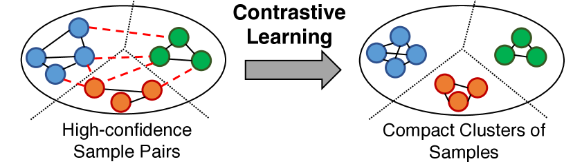
For samples from the same class, i.e. $W_{ij}=1$, Eq. 6 penalizes the distance between them, and for samples from different classes, the contrastive loss is large if their distance is small. In this way, the regularizer enforces similar samples to be close, while keeping dissimilar samples apart by at least $\gamma$. Figure 2 illustrates the contrastive representations. We can see that our method produces clear inter-class boundaries and small intra-class distances, which eases the classification tasks.

3.3 Confidence-based Sample Reweighting and Regularization

While contrastive representations yield better decision boundaries, they require samples with high-quality pseudo-labels. In this section, we introduce reweighting and regularization methods to suppress error propagation and refine pseudo-label qualities.

Sample Reweighting. In the classification task, samples with high prediction confidence are more likely to be classified correctly than those with low confidence. Therefore, we further reduce label noise propagation by a confidence-based sample reweighting scheme. For each sample $x$ with the soft pseudo-label $\widetilde{?}$, we assign $x$ with a weight $\omega (x)$ defined by

$$\omega =1-\frac{H\left(\widetilde{𝒚}\right)}{\log (C)},H(\widetilde{𝒚})=-\sum _{i=1}^C{\widetilde{𝒚}}_i\log {\widetilde{𝒚}}_i,$$ (8)

where $0\le H(\widetilde{?})\le \log (C)$ is the entropy of $\widetilde{?}$. Notice that if the prediction confidence is low, then $H(\widetilde{?})$ will be large, and the sample weight $\omega (x)$ will be small, and vice versa. We use a pre-defined threshold $\xi$ to select high confidence samples $?$ from each batch $ℬ$ as

$$𝒞=\{x\in ℬ|\omega (x)\ge \xi \}.$$ (9)

Then we define the loss function as

$${ℒ}_c(\theta ,\widetilde{𝒚})=\frac{1}{|𝒞|}\sum _{x\in 𝒞}\omega (x){𝒟}_{\mathrm{KL}}\left(\widetilde{𝒚}\parallel f(x;\theta )\right),$$ (10)

where

$${𝒟}_{\mathrm{KL}}(P\parallel Q)=\sum _k{p}_k\log \frac{p_k}{q_k}$$ (11)

is the Kullback–Leibler (KL) divergence.

Confidence regularization The sample reweighting approach promotes high confidence samples during contrastive self-training. However, this strategy relies on wrongly-labeled samples to have low confidence, which may not be true unless we prevent over-confident predictions. To this end, we propose a confidence-based regularizer that encourages smoothness over predictions, defined as

$${ℛ}_2(\theta )=\frac{1}{|𝒞|}\sum _{x\in 𝒞}{𝒟}_{\text{KL}}\left(𝐮\parallel f(x;\theta )\right),$$ (12)

where ${?}_{\text{KL}}$ is the KL-divergence and ${?}_i=1/C$ for $i=1,2,\mathrm{\cdots },C$. Such term constitutes a regularization to prevent over-confident predictions and leads to better generalization Pereyra et al. (2017).

4 Experiments

Datasets and Tasks. We conduct experiments on 6 NLP classification tasks using 7 public benchmarks: AGNews Zhang et al. (2015) is a Topic Classification task; IMDB Maas et al. (2011) and Yelp Meng et al. (2018) are Sentiment Analysis tasks; TREC Voorhees and Tice (1999) is a Question Classification task; MIT-R Liu et al. (2013) is a Slot Filling task; Chemprot Krallinger et al. (2017) is a Relation Classification task; and WiC Pilehvar and Camacho-Collados (2019) is a Word Sense Disambiguation (WSD) task. The dataset statistics are summarized in Table 2. More details on datasets and weak supervision sources are in Appendix A.

Dataset	Task	Class	# Train	# Dev	# Test	Cover	Accuracy
AGNews	Topic	4	96k	12k	12k	56.4	83.1
IMDB	Sentiment	2	20k	2.5k	2.5k	87.5	74.5
Yelp	Sentiment	2	30.4k	3.8k	3.8k	82.8	71.5
MIT-R	Slot Filling	9	6.6k	1.0k	1.5k	13.5	80.7
TREC	Question	6	4.8k	0.6k	0.6k	95.0	63.8
Chemprot	Relation	10	12.6k	1.6k	1.6k	85.9	46.5
WiC	WSD	2	5.4k	0.6k	1.4k	63.4	58.8

Table 2: Dataset statistics. Here cover (in %) is the fraction of instances covered by weak supervision sources in the training set, and accuracy (in %) is the precision of weak supervision.

Baselines. We compare our model with different groups of baseline methods:

(i) Exact Matching (ExMatch): The test set is directly labeled by weak supervision sources.

(ii) Fine-tuning Methods: The second group of baselines are fine-tuning methods for LMs:

$\diamond$RoBERTa Liu et al. (2019) uses the RoBERTa-base model with task-specific classification heads.

$\diamond$ Self-ensemble (Xu et al., 2020) uses self-ensemble and distillation to improve performances.

$\diamond$ FreeLB Zhu et al. (2020) adopts adversarial training to enforce smooth outputs.

$\diamond$ Mixup Zhang et al. (2018) creates virtual training samples by linear interpolations.

$\diamond$ SMART Jiang et al. (2020) adds adversarial and smoothness constraints to fine-tune LMs and achieves state-of-the-art result for many NLP tasks.

(iii) Weakly-supervised Models: The third group of baselines are weakly-supervised models:

$\diamond$ Snorkel Ratner et al. (2020) aggregates different labeling functions based on their correlations.

$\diamond$ WeSTClass Meng et al. (2018) trains a classifier with generated pseudo-documents and use self-training to bootstrap over all samples.

$\diamond$ ImplyLoss Awasthi et al. (2020) co-trains a rule-based classifier and a neural classifier to denoise.

$\diamond$ Denoise Ren et al. (2020) uses attention network to estimate reliability of weak supervisions, and then reduces the noise by aggregating weak labels.

$\diamond$ UST Mukherjee and Awadallah (2020) is state-of-the-art for self-training with limited labels. It estimates uncertainties via MC-dropout Gal and Ghahramani (2015), and then select samples with low uncertainties for self-training.

Evaluation Metrics. We use classification accuracy on the test set as the evaluation metric for all datasets except MIT-R. MIT-R contains a large number of tokens that are labeled as “Others”. We use the micro $F_1$ score from other classes for this dataset.

Auxiliary. We implement COSINE using PyTorch, and we use RoBERTa-base as the pre-trained LM. Datasets and weak supervision details are in Appendix A. Baseline settings are in Appendices B. Training details and setups are in Appendix C. Discussions on early-stopping are in Appendix D. Comparison of distance metrics and similarity measures are in Appendix E.

4.1 Learning From Weak Labels

Method	AGNews	IMDB	Yelp	MIT-R	TREC	Chemprot	WiC (dev)
ExMatch	$52.31$	$71.28$	$68.68$	$34.93$	$60.80$	$46.52$	$58.80$
Fully-supervised Result
RoBERTa-CL${}^{\diamond }$ Liu et al. (2019)	$91.41$	$94.26$	$97.27$	$88.51$	$96.68$	$79.65$	$70.53$
Baselines
RoBERTa-WL${}^{†}$ Liu et al. (2019)	$82.25$	$72.60$	$74.89$	$70.95$	$62.25$	$44.80$	$59.36$
Self-ensemble Xu et al. (2020)	$85.72$	$86.72$	$80.08$	$72.88$	$66.18$	$44.62$	$62.71$
FreeLB Zhu et al. (2020)	$85.12$	$88.04$	$85.68$	$73.04$	$67.33$	$45.68$	$63.45$
Mixup Zhang et al. (2018)	$85.40$	$86.92$	$92.05$	$73.68$	$66.83$	$51.59$	$64.88$
SMART Jiang et al. (2020)	$86.12$	$86.98$	$88.58$	$73.66$	$68.17$	$48.26$	$63.55$
Snorkel Ratner et al. (2020)	$62.91$	$73.22$	$69.21$	$20.63$	$58.60$	$37.50$	-​-​-${}^{\ast }$
WeSTClass Meng et al. (2018)	$82.78$	$77.40$	$76.86$	-​-​-${}^{\otimes }$	$37.31$	-​-​-${}^{\otimes }$	$48.59$
ImplyLoss Awasthi et al. (2020)	$68.50$	$63.85$	$76.29$	$74.30$	$80.20$	$53.48$	$54.48$
Denoise Ren et al. (2020)	$85.71$	$82.90$	$87.53$	$70.58$	$69.20$	$50.56$	$62.38$
UST Mukherjee and Awadallah (2020)	$86.28$	$84.56$	$90.53$	$74.41$	$65.52$	$52.14$	$63.48$
Our COSINE Framework
Init	$84.63$	$83.58$	$81.76$	$72.97$	$65.67$	$51.34$	$63.46$
COSINE	87.52	90.54	95.97	76.61	82.59	54.36	67.71

${}^{\diamond }$: RoBERTa is trained with clean labels. ${}^{†}$: RoBERTa is trained with weak labels. ${}^{\ast }$: unfair comparison. ${}^{\otimes }$: not applicable.

Table 3: Classification accuracy (in %) on various datasets. We report the mean over three runs.

We summarize the weakly-supervised leaning results in Table 3. In all the datasets, COSINE outperforms all the baseline models. A special case is the WiC dataset, where we use WordNet to generate weak labels. However, this enables Snorkel to access some labeled data in the development set, making it unfair to compete against other methods. We will discuss more about this dataset in Sec. 4.3.

In comparison with directly fine-tuning the pre-trained LMs with weakly-labeled data, our model employs an “earlier stopping” technique so that it does not overfit on the label noise. As shown, indeed “Init” achieves better performance, and it serves as a good initialization for our framework. Other fine-tuning methods and weakly-supervised models either cannot harness the power of pre-trained language models, e.g., Snorkel, or rely on clean labels, e.g., other baselines. We highlight that although UST, the state-of-the-art method to date, achieves strong performance under few-shot settings, their approach cannot estimate confidence well with noisy labels, and this yields inferior performance. Our model can gradually correct wrong pseudo-labels and mitigate error propagation via contrastive self-training.

It is worth noticing that on some datasets, e.g., AGNews, IMDB, Yelp, and WiC, our model achieves the same level of performance with models (RoBERTa-CL) trained with clean labels. This makes COSINE appealing in the scenario where only weak supervision is available.

Figure 3: Results of label corruption on TREC. When the corruption ratio is less than 40%, the performance is close to the fully supervised method.

4.2 Robustness Against Label Noise

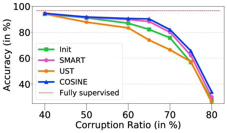
Our model is robust against excessive label noise. We corrupt certain percentage of labels by randomly changing each one of them to another class. This is a common scenario in crowd-sourcing, where we assume human annotators mis-label each sample with the same probability. Figure 3 summarizes experiment results on the TREC dataset. Compared with advanced fine-tuning and self-training methods (e.g. SMART and UST), our model consistently outperforms the baselines.

Model	Dev	Test	#Params
Human Baseline	80.0		-​-​-
BERT Devlin et al. (2019)	-​-​-	69.6	335M
RoBERTa (Liu et al., 2019)	70.5	69.9	356M
T5 (Raffel et al., 2019)	-​-​-	76.9	11,000M
Semi-Supervised Learning
SenseBERT (Levine et al., 2020)	-​-​-	72.1	370M
RoBERTa-WL${}^{†}$ (Liu et al., 2019)	72.3	70.2	125M
w/ MT${}^{†}$ (Tarvainen and Valpola, 2017)	73.5	70.9	125M
w/ VAT${}^{†}$ (Miyato et al., 2018)	74.2	71.2	125M
w/ COSINE${}^{\mathrm{†}}$	76.0	73.2	125M
Transductive Learning
Snorkel${}^{†}$ (Ratner et al., 2020)	80.5	-​-​-	1M
RoBERTa-WL${}^{†}$ (Liu et al., 2019)	81.3	76.8	125M
w/ MT${}^{†}$ (Tarvainen and Valpola, 2017)	82.1	77.1	125M
w/ VAT${}^{†}$ (Miyato et al., 2018)	84.9	79.5	125M
w/ COSINE${}^{\mathrm{†}}$	89.5	85.3	125M

Table 4: Semi-supervised Learning on WiC. VAT (Virtual Adversarial Training) and MT (Mean Teacher) are semi-supervised methods. ${}^{\mathrm{†}}$: has access to weak labels.

4.3 Semi-supervised Learning

We can naturally extend our model to semi-supervised learning, where clean labels are available for a portion of the data. We conduct experiments on the WiC dataset. As a part of the SuperGLUE Wang et al. (2019a) benchmark, this dataset proposes a challenging task: models need to determine whether the same word in different sentences has the same sense (meaning).

Different from previous tasks where the labels in the training set are noisy, in this part, we utilize the clean labels provided by the WiC dataset. We further augment the original training data of WiC with unlabeled sentence pairs obtained from lexical databases (e.g., WordNet, Wictionary). Note that part of the unlabeled data can be weakly-labeled by rule matching. This essentially creates a semi-supervised task, where we have labeled data, weakly-labeled data and unlabeled data.

Since the weak labels of WiC are generated by WordNet and partially reveal the true label information, Snorkel (Ratner et al., 2020) takes this unfair advantage by accessing the unlabeled sentences and weak labels of validation and test data. To make a fair comparison to Snorkel, we consider the transductive learning setting, where we are allowed access to the same information by integrating unlabeled validation and test data and their weak labels into the training set. As shown in Table 4, COSINE with transductive learning achieves better performance compared with Snorkel. Moreover, in comparison with semi-supervised baselines (i.e. VAT and MT) and fine-tuning methods with extra resources (i.e., SenseBERT), COSINE achieves better performance in both semi-supervised and transductive learning settings.

Figure 4: Classification performance on MIT-R. From left to right: visualization of ExMatch, results after the initialization step, results after contrastive self-training, and wrong-label correction during self-training.

Figure 5: Effects of different hyper-parameters.

(a) Effect of $\xi$. (b) Effect of $T_{\mathrm{1}}$. (c) Effect of $T_{\mathrm{3}}$.

Figure 5: Effects of different hyper-parameters.

Figure 6: Accuracy vs. Confidence score.

4.4 Case Study

(a) Embedding w/o ${ℛ}_{\mathrm{1}}$.

(b) Embedding w/ ${ℛ}_{\mathrm{1}}$.

Figure 7: t-SNE Maaten and Hinton (2008) visualization on TREC. Each color denotes a different class.

(a) Results on Agnews.

(b) Results on MIT-R.

Figure 8: Accuracy vs. Number of annotated labels.

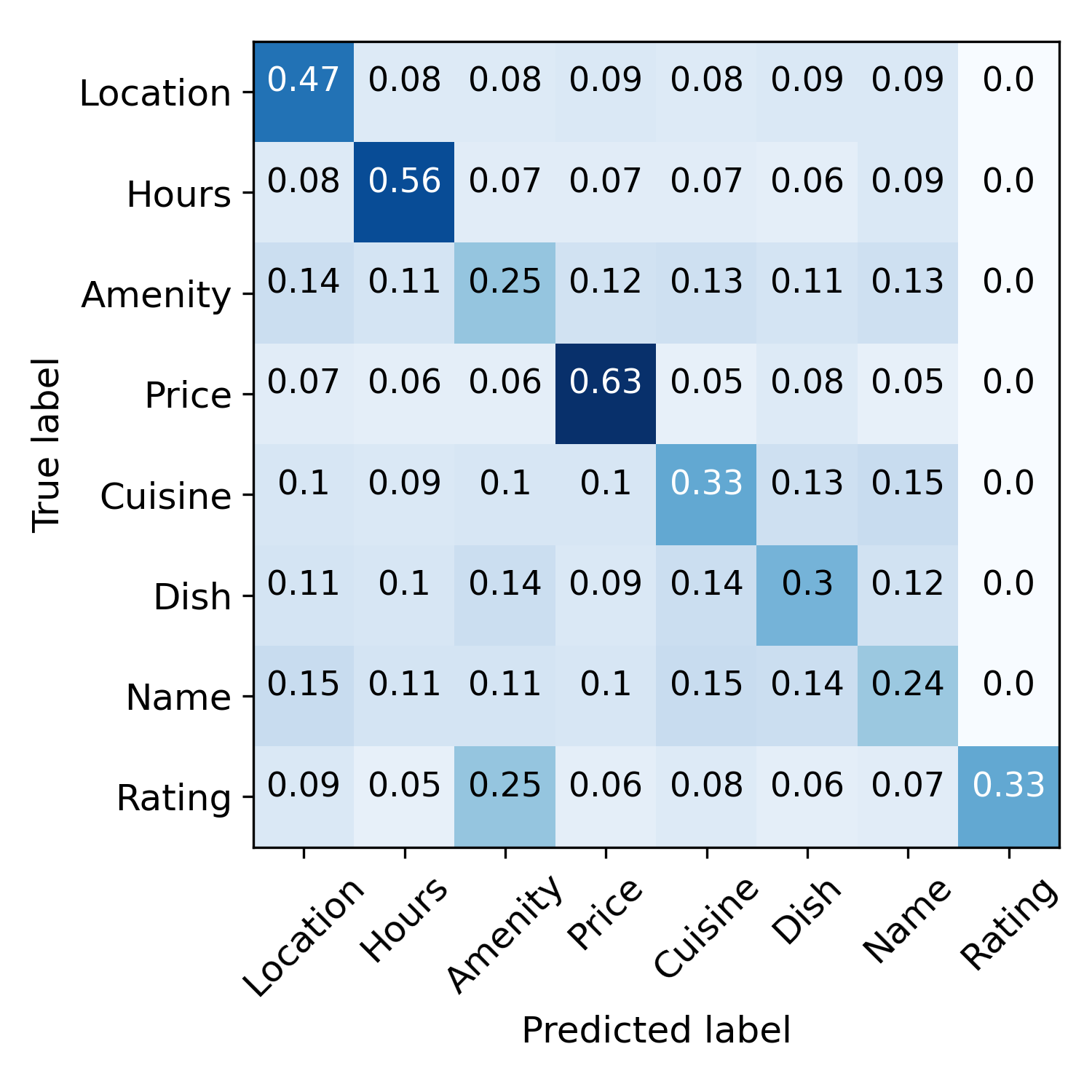
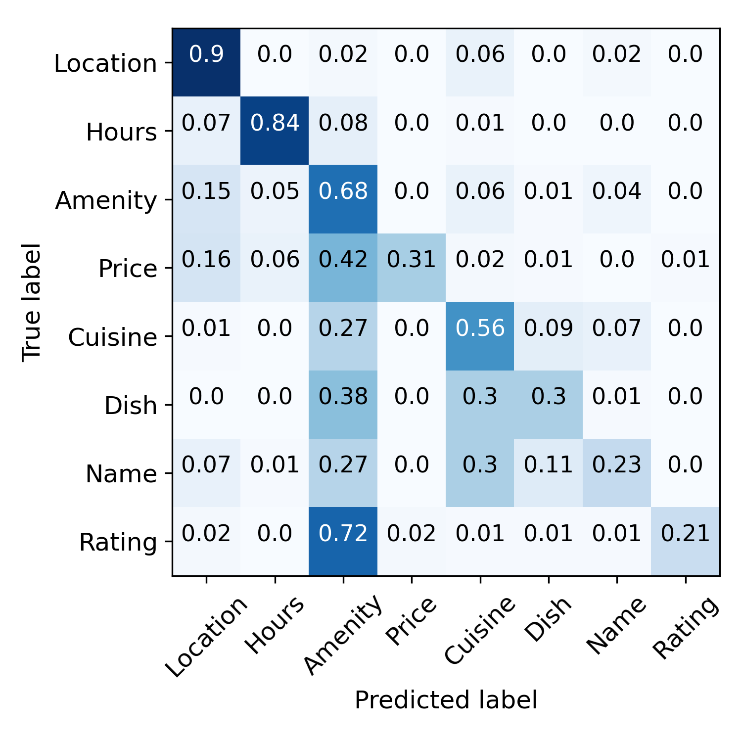
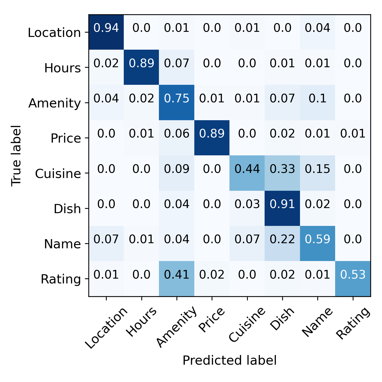
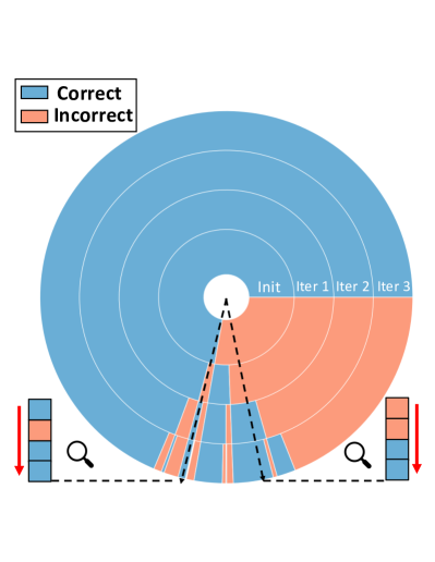
Error propagation mitigation and wrong-label correction. Figure 4 visualizes this process. Before training, the semantic rules make noisy predictions. After the initialization step, model predictions are less noisy but more biased, e.g., many samples are mis-labeled as “Amenity”. These predictions are further refined by contrastive self-training. The rightmost figure demonstrates wrong-label correction. Samples are indicated by radii of the circle, and classification correctness is indicated by color, i.e., blue means correct and orange means incorrect. From inner to outer tori specify classification accuracy after the initialization stage, and the iteration 1,2,3. We can see that many incorrect predictions are corrected within three iterations. To illustrate: the right black dashed line means the corresponding sample is classified correctly after the first iteration, and the left dashed line indicates the case where the sample is mis-classified after the second iteration but corrected after the third. These results demonstrate that our model can correct wrong predictions via contrastive self-training.

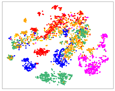
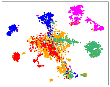
Better data representations. We visualize sample embeddings in Fig. 7. By incorporating the contrastive regularizer ${ℛ}_1$, our model learns more compact representations for data in the same class, e.g., the green class, and also extends the inter-class distances, e.g., the purple class is more separable from other classes in Fig. 7(b) than in Fig. 7(a).

Figure 9: Learning curves on TREC with different settings. Mean and variance are calculated over 3 runs.

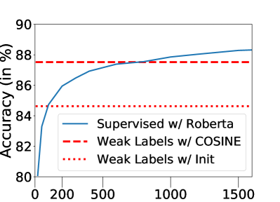
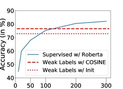
Label efficiency. Figure 8 illustrates the number of clean labels needed for the supervised model to outperform COSINE. On both of the datasets, the supervised model requires a significant amount of clean labels (around 750 for Agnews and 120 for MIT-R) to reach the level of performance as ours, whereas our method assumes no clean sample.

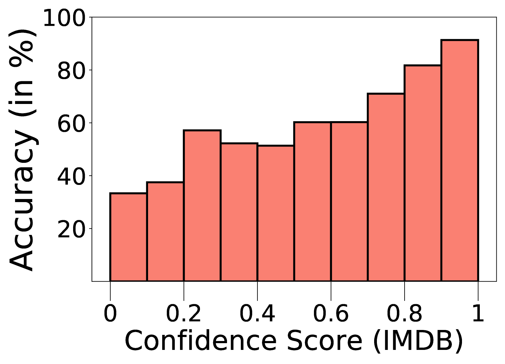
Higher Confidence Indicates Better Accuracy. Figure 6 demonstrates the relation between prediction confidence and prediction accuracy on IMDB. We can see that in general, samples with higher prediction confidence yield higher prediction accuracy. With our sample reweighting method, we gradually filter out low-confidence samples and assign higher weights for others, which effectively mitigates error propagation.

4.5 Ablation Study

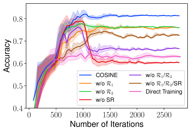
Components of COSINE. We inspect the importance of various components, including the contrastive regularizer ${ℛ}_1$, the confidence regularizer ${ℛ}_2$, and the sample reweighting (SR) method, and the soft labels. Table 5 summarizes the results and Fig. 9 visualizes the learning curves. We remark that all the components jointly contribute to the model performance, and removing any of them hurts the classification accuracy. For example, sample reweighting is an effective tool to reduce error propagation, and removing it causes the model to eventually overfit to the label noise, e.g., the red bottom line in Fig. 9 illustrates that the classification accuracy increases and then drops rapidly. On the other hand, replacing the soft pseudo-labels (Eq. 3) with the hard counterparts (Eq. 2) causes drops in performance. This is because hard pseudo-labels lose prediction confidence information.

Method	AGNews	IMDB	Yelp	MIT-R	TREC
Init	$84.63$	$83.58$	$81.76$	$72.97$	$66.50$
COSINE	87.52	90.54	95.97	76.61	82.59
w/o ${ℛ}_1$	$86.04$	$88.32$	$94.64$	$74.11$	$78.28$
w/o ${ℛ}_2$	$85.91$	$89.32$	$93.96$	$75.21$	$77.11$
w/o SR	$86.72$	$87.10$	$93.08$	$74.29$	$79.77$
w/o ${ℛ}_1$/${ℛ}_2$	$86.33$	$84.44$	$92.34$	$73.67$	$76.95$
w/o ${ℛ}_1$/${ℛ}_2$/SR	$86.61$	$83.98$	$82.57$	$73.59$	$74.96$
w/o Soft Label	$86.07$	$89.72$	$93.73$	$73.05$	$71.91$

Table 5: Effects of different components. Due to space limit we only show results for 5 representative datasets.

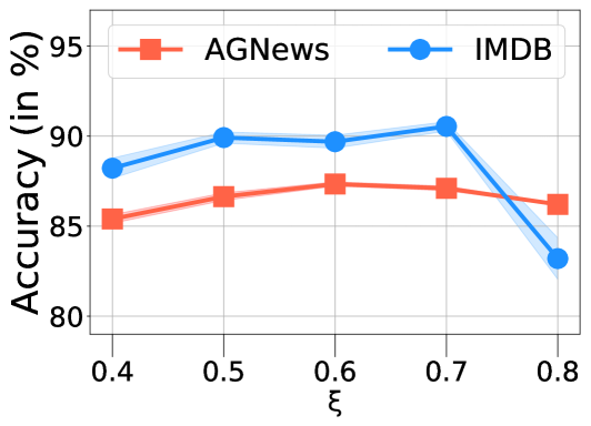
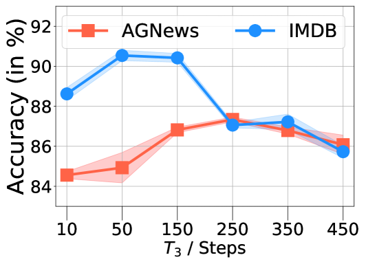
Hyper-parameters of COSINE. In Fig. 6, we examine the effects of different hyper-parameters, including the confidence threshold $\xi$ (Eq. 9), the stopping time $T_1$ in the initialization step, and the update period $T_3$ for pseudo-labels. From Fig. 5(a), we can see that setting the confidence threshold too big hurts model performance, which is because an over-conservative selection strategy can result in insufficient number of training data. The stopping time $T_1$ has drastic effects on the model. This is because fine-tuning COSINE with weak labels for excessive steps causes the model to unavoidably overfit to the label noise, such that the contrastive self-training procedure cannot correct the error. Also, with the increment of $T_3$, the update period of pseudo-labels, model performance first increases and then decreases. This is because if we update pseudo-labels too frequently, the contrastive self-training procedure cannot fully suppress the label noise, and if the updates are too infrequent, the pseudo-labels cannot capture the updated information well.

5 Related Works

Fine-tuning Pre-trained Language Models. To improve the model’s generalization power during fine-tuning stage, several methods are proposed Peters et al. (2019); Dodge et al. (2020); Zhu et al. (2020); Jiang et al. (2020); Xu et al. (2020); Kong et al. (2020); Zhao et al. (2020); Gunel et al. (2021); Zhang et al. (2021); Aghajanyan et al. (2021); Wang et al. (2021), However, most of these methods focus on fully-supervised setting and rely heavily on large amounts of clean labels, which are not always available. To address this issue, we propose a contrastive self-training framework that fine-tunes pre-trained models with only weak labels. Compared with the existing fine-tuning approaches Xu et al. (2020); Zhu et al. (2020); Jiang et al. (2020), our model effectively reduce the label noise, which achieves better performance on various NLP tasks with weak supervision.

Learning From Weak Supervision. In weakly-supervised learning, the training data are usually noisy and incomplete. Existing methods aim to denoise the sample labels or the labeling functions by, for example, aggregating multiple weak supervisions Ratner et al. (2020); Lison et al. (2020); Ren et al. (2020), using clean samples Awasthi et al. (2020), and leveraging contextual information Mekala and Shang (2020). However, most of them can only use specific type of weak supervision on specific task, e.g., keywords for text classification Meng et al. (2020); Mekala and Shang (2020), and they require prior knowledge on weak supervision sources Awasthi et al. (2020); Lison et al. (2020); Ren et al. (2020), which somehow limits the scope of their applications. Our work is orthogonal to them since we do not denoise the labeling functions directly. Instead, we adopt contrastive self-training to leverage the power of pre-trained language models for denoising, which is task-agnostic and applicable to various NLP tasks with minimal additional efforts.

6 Discussions

Adaptation of LMs to Different Domains. When fine-tuning LMs on data from different domains, we can first continue pre-training on in-domain text data for better adaptation Gururangan et al. (2020). For some rare domains where BERT trained on general domains is not optimal, we can use LMs pretrained on those specific domains (e.g. BioBERT Lee et al. (2020), SciBERT Beltagy et al. (2019)) to tackle this issue.

Scalability of Weak Supervision. COSINE can be applied to tasks with a large number of classes. This is because rules can be automatically generated beyond hand-crafting. For example, we can use label names/descriptions as weak supervision signals Meng et al. (2020). Such signals are easy to obtain and do not require hand-crafted rules. Once weak supervision is provided, we can create weak labels to further apply COSINE.

Flexibility. COSINE can handle tasks and weak supervision sources beyond our conducted experiments. For example, other than semantic rules, crowd-sourcing can be another weak supervision source to generate pseudo-labels Wang et al. (2013). Moreover, we only conduct experiments on several representative tasks, but our framework can be applied to other tasks as well, e.g., named-entity recognition (token classification) and reading comprehension (sentence pair classification).

7 Conclusion

In this paper, we propose a contrastive regularized self-training framework, COSINE, for fine-tuning pre-trained language models with weak supervision. Our framework can learn better data representations to ease the classification task, and also efficiently reduce label noise propagation by confidence-based reweighting and regularization. We conduct experiments on various classification tasks, including sequence classification, token classification, and sentence pair classification, and the results demonstrate the efficacy of our model.

Broader Impact

COSINE is a general framework that tackled the label scarcity issue via combining neural nets with weak supervision. The weak supervision provides a simple but flexible language to encode the domain knowledge and capture the correlations between features and labels. When combined with unlabeled data, our framework can largely tackle the label scarcity bottleneck for training DNNs, enabling them to be applied for downstream NLP classification tasks in a label efficient manner.

COSINE neither introduces any social/ethical bias to the model nor amplify any bias in the data. In all the experiments, we use publicly available data, and we build our algorithms using public code bases. We do not foresee any direct social consequences or ethical issues.

Appendix A Weak Supervision Details

COSINE does not require any human annotated examples in the training process, and it only needs weak supervision sources such as keywords and semantic rules. According to some studies in existing works Awasthi et al. (2020); Zhou et al. (2020), such weak supervisions are cheap to obtain and are much efficient than collecting clean labels. In this way, we can obtain significantly more labeled examples using these weak supervision sources than human labor.

There are two types of semantic rules that we apply as weak supervisions:

1. Keyword Rule: HAS(x, L) $\mathrm{\to }$ C. If $x$ matches one of the words in the list $L$, we label it as $C$.

2. Pattern Rule: MATCH(x, R) $\mathrm{\to }$ C. If $x$ matches the regular expression $R$, we label it as $C$.

In addition to the keyword rule and the pattern rule, we can also use third-party tools to obtain weak labels. These tools (e.g. TextBlob) are available online and can be obtained cheaply, but their prediction is not accurate enough (when directly use this tool to predict label for all training samples, the accuracy on Yelp dataset is around 60%).
We now introduce the semantic rules on each dataset:

1. AGNews, IMDB, Yelp: We use the rule in Ren et al. (2020). Please refer to the original paper for detailed information on rules.

2. MIT-R, TREC: We use the rule in Awasthi et al. (2020). Please refer to the original paper for detailed information on rules.

3. ChemProt: There are 26 rules. We show part of the rules in Table 6.

4. WiC: Each sense of each word in WordNet has example sentences. For each sentence in the WiC dataset and its corresponding keyword, we collect the example sentences of that word from WordNet. Then for a pair of sentences, the corresponding weak label is “True” if their definitions are the same, otherwise the weak label is “False”.

Rule	Example
HAS (x, [amino acid,mutant, mutat, replace] ) $\mathrm{\to }$ part_of	A major part of this processing requires endoproteolytic cleavage at specific pairs of basic [CHEMICAL]amino acid[CHEMICAL] residues, an event necessary for the maturation of a variety of important biologically active proteins, such as insulin and [GENE]nerve growth factor[GENE].
HAS (x, [bind, interact, affinit] ) $\mathrm{\to }$ regulator	The interaction of [CHEMICAL]naloxone estrone azine[CHEMICAL] (N-EH) with various [GENE]opioid receptor[GENE] types was studied in vitro.
HAS (x, [activat, increas, induc, stimulat, upregulat] ) $\mathrm{\to }$ upregulator/activator	The results of this study suggest that [CHEMICAL]noradrenaline[CHEMICAL] predominantly, but not exclusively, mediates contraction of rat aorta through the activation of an [GENE]alphalD-adrenoceptor[GENE].
HAS (x, [downregulat, inhibit, reduc, decreas] ) $\mathrm{\to }$ downregulator/inhibitor	These results suggest that [CHEMICAL]prostacyclin[CHEMICAL] may play a role in downregulating [GENE]tissue factor[GENE] expression in monocytes, at least in part via elevation of intracellular levels of cyclic AMP.
HAS (x, [ agoni, tagoni]* ) $\mathrm{\to }$ agonist * (note the leading whitespace in both cases)	Alprenolol and BAAM also caused surmountable antagonism of [CHEMICAL]isoprenaline[CHEMICAL] responses, and this [GENE]beta 1-adrenoceptor[GENE] antagonism was slowly reversible.
HAS (x, [antagon] ) $\mathrm{\to }$ antagonist	It is concluded that [CHEMICAL]labetalol[CHEMICAL] and dilevalol are [GENE]beta 1-adrenoceptor[GENE] selective antagonists.
HAS (x, [modulat, allosteric] ) $\mathrm{\to }$ modulator	[CHEMICAL]Hydrogen sulfide[CHEMICAL] as an allosteric modulator of [GENE]ATP-sensitive potassium channels[GENE] in colonic inflammation.
HAS (x, [cofactor] ) $\mathrm{\to }$ cofactor	The activation appears to be due to an increase of [GENE]GAD[GENE] affinity for its cofactor, [CHEMICAL]pyridoxal phosphate[CHEMICAL] (PLP).
HAS (x, [substrate, catalyz, transport, produc, conver] ) $\mathrm{\to }$ substrate/product	Kinetic constants of the mutant [GENE]CrAT[GENE] showed modification in favor of longer [CHEMICAL]acyl-CoAs[CHEMICAL] as substrates.
HAS (x, [not] ) $\mathrm{\to }$ not	[CHEMICAL]Nicotine[CHEMICAL] does not account for the CSE stimulation of [GENE]VEGF[GENE] in HFL-1.

Table 6: Examples of semantic rules on Chemprot.

Appendix B Baseline Settings

We implement Self-ensemble, FreeLB, Mixup and UST based on their original paper. For other baselines, we use their official release:
$\diamond$ WeSTClass Meng et al. (2018): https://github.com/yumeng5/WeSTClass.
$\diamond$ RoBERTa Liu et al. (2019): https://github.com/huggingface/transformers.
$\diamond$ SMART Jiang et al. (2020): https://github.com/namisan/mt-dnn.
$\diamond$ Snorkel Ratner et al. (2020): https://www.snorkel.org/.
$\diamond$ ImplyLoss Awasthi et al. (2020): https://github.com/awasthiabhijeet/Learning-From-Rules.
$\diamond$ Denoise Ren et al. (2020): https://github.com/weakrules/Denoise-multi-weak-sources.

Appendix C Details on Experiment Setups

C.1 Computing Infrastructure

System: Ubuntu 18.04.3 LTS; Python 3.7; Pytorch 1.2. CPU: Intel(R) Core(TM) i7-5930K CPU @ 3.50GHz. GPU: GeForce GTX TITAN X.

C.2 Hyper-parameters

We use AdamW Loshchilov and Hutter (2019) as the optimizer, and the learning rate is chosen from $1\times {10}^{-5},2\times {10}^{-5},3\times {10}^{-5}\}$. A linear learning rate decay schedule with warm-up $0.1$ is used, and the number of training epochs is $5$.

Hyper-parameters are shown in Table 7. We use a grid search to find the optimal setting for each task. Specifically, we search $T_1$ from $10$ to $2000$, $T_2$ from $1000$ to $5000$, $T_3$ from $10$ to $500$, $\xi$ from $0$, and $\lambda$ from $0$. All results are reported as the average over three runs.

Hyper-parameter	AGNews	IMDB	Yelp	MIT-R	TREC	Chemprot	WiC
Dropout Ratio	0.1
Maximum Tokens	128	256	512	64	64	400	256
Batch Size	32	16	16	64	16	24	32
Weight Decay	${10}^{-4}$
Learning Rate	${10}^{-5}$	${10}^{-5}$	${10}^{-5}$	${10}^{-5}$	${10}^{-5}$	${10}^{-5}$	${10}^{-5}$
$T_1$	160	160	200	150	500	400	1700
$T_2$	3000	2500	2500	1000	2500	1000	3000
$T_3$	250	50	100	15	30	15	80
$\xi$	0.6	0.7	0.7	0.2	0.3	0.7	0.7
$\lambda$	0.1	0.05	0.05	0.1	0.05	0.05	0.05

Table 7: Hyper-parameter configurations. Note that we only keep certain number of tokens.

C.3 Number of Parameters

COSINE and most of the baselines (RoBERTa-WL / RoBERTa-CL / SMART / WeSTClass / Self-Ensemble / FreeLB / Mixup / UST) are built on the RoBERTa-base model with about 125M parameters. Snorkel is a generative model with only a few parameters. ImplyLoss and Denoise freezes the embedding and has less than 1M parameters. However, these models cannot achieve satisfactory performance in our experiments.

Distance $d$	Euclidean			Cos
Similarity $W$	Hard	KL-based	L2-based	Hard	KL-based	L2-based
AGNews	87.52	86.44	86.72	87.34	86.98	86.55
MIT-R	76.61	76.68	76.49	76.55	76.76	76.58

Table 8: Performance of COSINE under different settings.

Appendix D Early Stopping and Earlier Stopping

Our model adopts the earlier stopping strategy during the initialization stage. Here we use “earlier stopping” to differentiate from “early stopping”, which is standard in fine-tuning algorithms. Early stopping refers to the technique where we stop training when the evaluation score drops. Earlier stopping is self-explanatory, namely we fine-tune the pre-trained LMs with only a few steps, even before the evaluation score starts dropping. This technique can efficiently prevent the model from overfitting. For example, as Figure 5(b) illustrates, on IMDB dataset, our model overfits after 240 iterations of initialization with weak labels. In contrast, the model achieves good performance even after 400 iterations of fine-tuning when using clean labels. This verifies the necessity of earlier stopping.

Appendix E Comparison of Distance Measures in Contrastive Learning

The contrastive regularizer ${ℛ}_1(\theta ;\widetilde{?})$ is related to two designs: the sample distance metric $d_{ij}$ and the sample similarity measure $W_{ij}$. In our implementation, we use the scaled Euclidean distance as the default for $d_{ij}$ and Eq. 5 as the default for $W_{ij}$. Here we discuss other designs.

E.1 Sample distance metric $d$

Given the encoded vectorized representations ${?}_i$ and ${?}_j$ for samples $i$ and $j$, we consider two distance metrics as follows.

Scaled Euclidean distance (Euclidean): We calculate the distance between ${?}_i$ and ${?}_j$ as

$$d_{ij}=\frac{1}{d}{\Vert {𝒗}_i-{𝒗}_j\Vert }_2^2.$$ (13)

Cosine distance (Cos): Besides the scaled Euclidean distance, cosine distance is another widely-used distance metric:

$$d_{ij}=1-\text{cos}({𝒗}_i,{𝒗}_j)=1-\frac{\Vert {𝒗}_i\cdot {𝒗}_j\Vert }{\Vert {𝒗}_i\Vert \Vert {𝒗}_j\Vert }.$$ (14)

E.2 Sample similarity measures $W$

Given the soft pseudo-labels ${\widetilde{?}}_i$ and ${\widetilde{?}}_j$ for samples $i$ and $j$, the following are some designs for $W_{ij}$. In all of the cases, $W_{ij}$ is scaled into range $[0,1]$ (we set $\gamma =1$ in Eq. 7 for the hard similarity).

Hard Similarity: The hard similarity between two samples is calculated as

(15)

This is called a “hard” similarity because we obtain a binary label, i.e., we say two samples are similar if their corresponding hard pseudo-labels are the same, otherwise we say they are dissimilar.

Soft KL-based Similarity: We calculate the similarity based on KL distance as follows.

$$W_{ij}=\exp \left(-\frac{\beta }{2}\left({𝒟}_{KL}({\widetilde{𝒚}}_i\parallel {\widetilde{𝒚}}_j)+{𝒟}_{KL}({\widetilde{𝒚}}_j\parallel {\widetilde{𝒚}}_i)\right)\right),$$ (16)

where $\beta$ is a scaling factor, and we set $\beta =10$ by default.

Soft L2-based Similarity: We calculate the similarity based on L2 distance as follows.

$$W_{ij}=1-\frac{1}{2}{\Vert {\widetilde{𝒚}}_i-{\widetilde{𝒚}}_j\Vert }_2^2,$$ (17)

E.3 COSINE under different $d$ and $W$.

We show the performance of COSINE with different choices of $d$ and $W$ on Agnews and MIT-R in Table 8. We can see that COSINE is robust to these choices. In our experiments, we use the scaled euclidean distance and the hard similarity by default.

References

- Aghajanyan et al. (2021) Armen Aghajanyan, Akshat Shrivastava, Anchit Gupta, Naman Goyal, Luke Zettlemoyer, and Sonal Gupta. 2021. Better fine-tuning by reducing representational collapse. In International Conference on Learning Representations.
- Aina et al. (2019) Laura Aina, Kristina Gulordava, and Gemma Boleda. 2019. Putting words in context: LSTM language models and lexical ambiguity. In Proceedings of the 57th Annual Meeting of the Association for Computational Linguistics, pages 3342–3348.
- Awasthi et al. (2020) Abhijeet Awasthi, Sabyasachi Ghosh, Rasna Goyal, and Sunita Sarawagi. 2020. Learning from rules generalizing labeled exemplars. In International Conference on Learning Representations.
- Beltagy et al. (2019) Iz Beltagy, Kyle Lo, and Arman Cohan. 2019. SciBERT: A pretrained language model for scientific text. In Proceedings of the 2019 Conference on Empirical Methods in Natural Language Processing and the 9th International Joint Conference on Natural Language Processing (EMNLP-IJCNLP), pages 3615–3620.
- Chopra et al. (2005) Sumit Chopra, Raia Hadsell, and Yann LeCun. 2005. Learning a similarity metric discriminatively, with application to face verification. In IEEE Conference on Computer Vision and Pattern Recognition (CVPR’05), volume 1, pages 539–546.
- Devlin et al. (2019) Jacob Devlin, Ming-Wei Chang, Kenton Lee, and Kristina Toutanova. 2019. BERT: Pre-training of deep bidirectional transformers for language understanding. In Proceedings of the 2019 Conference of the North American Chapter of the Association for Computational Linguistics: Human Language Technologies, Volume 1 (Long and Short Papers), pages 4171–4186.
- Dodge et al. (2020) Jesse Dodge, Gabriel Ilharco, Roy Schwartz, Ali Farhadi, Hannaneh Hajishirzi, and Noah A. Smith. 2020. Fine-tuning pretrained language models: Weight initializations, data orders, and early stopping. CoRR, abs/2002.06305.
- Gal and Ghahramani (2015) Yarin Gal and Zoubin Ghahramani. 2015. Bayesian convolutional neural networks with bernoulli approximate variational inference. CoRR, abs/1506.02158.
- Gunel et al. (2021) Beliz Gunel, Jingfei Du, Alexis Conneau, and Veselin Stoyanov. 2021. Supervised contrastive learning for pre-trained language model fine-tuning. In International Conference on Learning Representations.
- Gururangan et al. (2020) Suchin Gururangan, Ana Marasović, Swabha Swayamdipta, Kyle Lo, Iz Beltagy, Doug Downey, and Noah A. Smith. 2020. Don’t stop pretraining: Adapt language models to domains and tasks. In Proceedings of the 58th Annual Meeting of the Association for Computational Linguistics, pages 8342–8360.
- Jiang et al. (2020) Haoming Jiang, Pengcheng He, Weizhu Chen, Xiaodong Liu, Jianfeng Gao, and Tuo Zhao. 2020. SMART: Robust and efficient fine-tuning for pre-trained natural language models through principled regularized optimization. In Proceedings of the 58th Annual Meeting of the Association for Computational Linguistics, pages 2177–2190.
- Kong et al. (2020) Lingkai Kong, Haoming Jiang, Yuchen Zhuang, Jie Lyu, Tuo Zhao, and Chao Zhang. 2020. Calibrated language model fine-tuning for in- and out-of-distribution data. In Proceedings of the 2020 Conference on Empirical Methods in Natural Language Processing (EMNLP), pages 1326–1340.
- Krallinger et al. (2017) Martin Krallinger, Obdulia Rabal, Saber A Akhondi, et al. 2017. Overview of the biocreative VI chemical-protein interaction track. In Proceedings of the sixth BioCreative challenge evaluation workshop, volume 1, pages 141–146.
- Lee (2013) Dong-Hyun Lee. 2013. Pseudo-label: The simple and efficient semi-supervised learning method for deep neural networks. In Workshop on challenges in representation learning, ICML, volume 3, page 2.
- Lee et al. (2020) Jinhyuk Lee, Wonjin Yoon, Sungdong Kim, Donghyeon Kim, Sunkyu Kim, Chan Ho So, and Jaewoo Kang. 2020. Biobert: a pre-trained biomedical language representation model for biomedical text mining. Bioinformatics, 36(4):1234–1240.
- Levine et al. (2020) Yoav Levine, Barak Lenz, Or Dagan, Ori Ram, Dan Padnos, Or Sharir, Shai Shalev-Shwartz, Amnon Shashua, and Yoav Shoham. 2020. SenseBERT: Driving some sense into BERT. In Proceedings of the 58th Annual Meeting of the Association for Computational Linguistics, pages 4656–4667.
- Liang et al. (2020) Chen Liang, Yue Yu, Haoming Jiang, Siawpeng Er, Ruijia Wang, Tuo Zhao, and Chao Zhang. 2020. Bond: Bert-assisted open-domain named entity recognition with distant supervision. In Proceedings of the 26th ACM SIGKDD International Conference on Knowledge Discovery & Data Mining, page 1054–1064.
- Lison et al. (2020) Pierre Lison, Jeremy Barnes, Aliaksandr Hubin, and Samia Touileb. 2020. Named entity recognition without labelled data: A weak supervision approach. In Proceedings of the 58th Annual Meeting of the Association for Computational Linguistics, pages 1518–1533.
- Liu et al. (2013) Jingjing Liu, Panupong Pasupat, Yining Wang, Scott Cyphers, and James R. Glass. 2013. Query understanding enhanced by hierarchical parsing structures. In 2013 IEEE Workshop on Automatic Speech Recognition and Understanding, pages 72–77. IEEE.
- Liu et al. (2019) Yinhan Liu, Myle Ott, Naman Goyal, Jingfei Du, Mandar Joshi, Danqi Chen, Omer Levy, Mike Lewis, Luke Zettlemoyer, and Veselin Stoyanov. 2019. Roberta: A robustly optimized BERT pretraining approach. CoRR, abs/1907.11692.
- Loshchilov and Hutter (2019) Ilya Loshchilov and Frank Hutter. 2019. Decoupled weight decay regularization. In International Conference on Learning Representations.
- Luo et al. (2017) Bingfeng Luo, Yansong Feng, Zheng Wang, Zhanxing Zhu, Songfang Huang, Rui Yan, and Dongyan Zhao. 2017. Learning with noise: Enhance distantly supervised relation extraction with dynamic transition matrix. In Proceedings of the 55th Annual Meeting of the Association for Computational Linguistics (Volume 1: Long Papers), pages 430–439.
- Maas et al. (2011) Andrew L. Maas, Raymond E. Daly, Peter T. Pham, Dan Huang, Andrew Y. Ng, and Christopher Potts. 2011. Learning word vectors for sentiment analysis. In Proceedings of the 49th Annual Meeting of the Association for Computational Linguistics: Human Language Technologies, pages 142–150.
- Maaten and Hinton (2008) Laurens van der Maaten and Geoffrey Hinton. 2008. Visualizing data using t-sne. Journal of machine learning research, 9(Nov):2579–2605.
- Mekala and Shang (2020) Dheeraj Mekala and Jingbo Shang. 2020. Contextualized weak supervision for text classification. In Proceedings of the 58th Annual Meeting of the Association for Computational Linguistics, pages 323–333.
- Meng et al. (2018) Yu Meng, Jiaming Shen, Chao Zhang, and Jiawei Han. 2018. Weakly-supervised neural text classification. In Proceedings of the 27th ACM International Conference on Information and Knowledge Management, page 983–992.
- Meng et al. (2020) Yu Meng, Yunyi Zhang, Jiaxin Huang, Chenyan Xiong, Heng Ji, Chao Zhang, and Jiawei Han. 2020. Text classification using label names only: A language model self-training approach. In Proceedings of the 2020 Conference on Empirical Methods in Natural Language Processing (EMNLP), pages 9006–9017.
- Miyato et al. (2018) Takeru Miyato, Shin-ichi Maeda, Masanori Koyama, and Shin Ishii. 2018. Virtual adversarial training: a regularization method for supervised and semi-supervised learning. IEEE transactions on pattern analysis and machine intelligence, 41(8):1979–1993.
- Mukherjee and Awadallah (2020) Subhabrata Mukherjee and Ahmed Hassan Awadallah. 2020. Uncertainty-aware self-training for text classification with few labels. CoRR, abs/2006.15315.
- Pereyra et al. (2017) Gabriel Pereyra, George Tucker, Jan Chorowski, Lukasz Kaiser, and Geoffrey E. Hinton. 2017. Regularizing neural networks by penalizing confident output distributions. CoRR, abs/1701.06548.
- Peters et al. (2018) Matthew Peters, Mark Neumann, Mohit Iyyer, Matt Gardner, Christopher Clark, Kenton Lee, and Luke Zettlemoyer. 2018. Deep contextualized word representations. In Proceedings of the 2018 Conference of the North American Chapter of the Association for Computational Linguistics: Human Language Technologies, Volume 1 (Long Papers), pages 2227–2237.
- Peters et al. (2019) Matthew E. Peters, Sebastian Ruder, and Noah A. Smith. 2019. To tune or not to tune? adapting pretrained representations to diverse tasks. In Proceedings of the 4th Workshop on Representation Learning for NLP (RepL4NLP-2019), pages 7–14.
- Pilehvar and Camacho-Collados (2019) Mohammad Taher Pilehvar and Jose Camacho-Collados. 2019. WiC: the word-in-context dataset for evaluating context-sensitive meaning representations. In Proceedings of the 2019 Conference of the North American Chapter of the Association for Computational Linguistics: Human Language Technologies, Volume 1 (Long and Short Papers), pages 1267–1273.
- Raffel et al. (2019) Colin Raffel, Noam Shazeer, Adam Roberts, Katherine Lee, Sharan Narang, Michael Matena, Yanqi Zhou, Wei Li, and Peter J. Liu. 2019. Exploring the limits of transfer learning with a unified text-to-text transformer. CoRR, abs/1910.10683.
- Ratner et al. (2020) Alexander Ratner, Stephen H. Bach, Henry R. Ehrenberg, Jason A. Fries, Sen Wu, and Christopher Ré. 2020. Snorkel: rapid training data creation with weak supervision. VLDB Journal, 29(2):709–730.
- Ren et al. (2020) Wendi Ren, Yinghao Li, Hanting Su, David Kartchner, Cassie Mitchell, and Chao Zhang. 2020. Denoising multi-source weak supervision for neural text classification. In Findings of the Association for Computational Linguistics: EMNLP 2020, pages 3739–3754.
- Rosenberg et al. (2005) Chuck Rosenberg, Martial Hebert, and Henry Schneiderman. 2005. Semi-supervised self-training of object detection models. WACV/MOTION, 2.
- Taigman et al. (2014) Yaniv Taigman, Ming Yang, Marc’Aurelio Ranzato, and Lior Wolf. 2014. Deepface: Closing the gap to human-level performance in face verification. In The IEEE Conference on Computer Vision and Pattern Recognition (CVPR).
- Tarvainen and Valpola (2017) Antti Tarvainen and Harri Valpola. 2017. Mean teachers are better role models: Weight-averaged consistency targets improve semi-supervised deep learning results. In Advances in Neural Information Processing Systems, pages 1195–1204.
- Varma and Ré (2018) Paroma Varma and Christopher Ré. 2018. Snuba: Automating weak supervision to label training data. Proc. VLDB Endowment, 12(3):223–236.
- Voorhees and Tice (1999) Ellen M. Voorhees and Dawn M. Tice. 1999. The TREC-8 question answering track evaluation. In Proceedings of The Eighth Text REtrieval Conference, volume 500-246.
- Wang et al. (2019a) Alex Wang, Yada Pruksachatkun, Nikita Nangia, Amanpreet Singh, Julian Michael, Felix Hill, Omer Levy, and Samuel Bowman. 2019a. Superglue: A stickier benchmark for general-purpose language understanding systems. In Advances in Neural Information Processing Systems, pages 3261–3275.
- Wang et al. (2013) Aobo Wang, Cong Duy Vu Hoang, and Min-Yen Kan. 2013. Perspectives on crowdsourcing annotations for natural language processing. Language resources and evaluation, 47(1):9–31.
- Wang et al. (2021) Boxin Wang, Shuohang Wang, Yu Cheng, Zhe Gan, Ruoxi Jia, Bo Li, and Jingjing Liu. 2021. InfoBERT: Improving robustness of language models from an information theoretic perspective. In International Conference on Learning Representations.
- Wang et al. (2019b) Hao Wang, Bing Liu, Chaozhuo Li, Yan Yang, and Tianrui Li. 2019b. Learning with noisy labels for sentence-level sentiment classification. In Proceedings of the 2019 Conference on Empirical Methods in Natural Language Processing and the 9th International Joint Conference on Natural Language Processing (EMNLP-IJCNLP), pages 6286–6292.
- Xie et al. (2016) Junyuan Xie, Ross Girshick, and Ali Farhadi. 2016. Unsupervised deep embedding for clustering analysis. In Proceedings of The 33rd International Conference on Machine Learning, pages 478–487.
- Xie et al. (2019) Qizhe Xie, Zihang Dai, Eduard H. Hovy, Minh-Thang Luong, and Quoc V. Le. 2019. Unsupervised data augmentation for consistency training. CoRR, abs/1904.12848.
- Xu et al. (2020) Yige Xu, Xipeng Qiu, Ligao Zhou, and Xuanjing Huang. 2020. Improving BERT fine-tuning via self-ensemble and self-distillation. CoRR, abs/2002.10345.
- Zhang et al. (2018) Hongyi Zhang, Moustapha Cisse, Yann N. Dauphin, and David Lopez-Paz. 2018. mixup: Beyond empirical risk minimization. In International Conference on Learning Representations.
- Zhang et al. (2021) Tianyi Zhang, Felix Wu, Arzoo Katiyar, Kilian Q Weinberger, and Yoav Artzi. 2021. Revisiting few-sample BERT fine-tuning. In International Conference on Learning Representations.
- Zhang et al. (2015) Xiang Zhang, Junbo Zhao, and Yann LeCun. 2015. Character-level convolutional networks for text classification. In Advances in Neural Information Processing Systems 28, pages 649–657.
- Zhao et al. (2020) Mengjie Zhao, Tao Lin, Fei Mi, Martin Jaggi, and Hinrich Schütze. 2020. Masking as an efficient alternative to finetuning for pretrained language models. In Proceedings of the 2020 Conference on Empirical Methods in Natural Language Processing (EMNLP), pages 2226–2241.
- Zhou et al. (2020) Wenxuan Zhou, Hongtao Lin, Bill Yuchen Lin, Ziqi Wang, Junyi Du, Leonardo Neves, and Xiang Ren. 2020. NERO: A neural rule grounding framework for label-efficient relation extraction. In Proceedings of The Web Conference 2020, page 2166–2176.
- Zhu et al. (2020) Chen Zhu, Yu Cheng, Zhe Gan, Siqi Sun, Tom Goldstein, and Jingjing Liu. 2020. Freelb: Enhanced adversarial training for natural language understanding. In International Conference on Learning Representations.