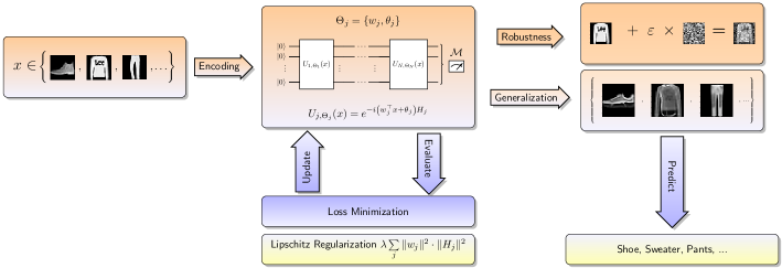
Training robust and generalizable quantum models

Abstract

Adversarial robustness and generalization are both crucial properties of reliable machine learning models. In this paper, we study these properties in the context of quantum machine learning based on Lipschitz bounds. We derive tailored, parameter-dependent Lipschitz bounds for quantum models with trainable encoding, showing that the norm of the data encoding has a crucial impact on the robustness against perturbations in the input data. Further, we derive a bound on the generalization error which explicitly depends on the parameters of the data encoding. Our theoretical findings give rise to a practical strategy for training robust and generalizable quantum models by regularizing the Lipschitz bound in the cost. Further, we show that, for fixed and non-trainable encodings as frequently employed in quantum machine learning, the Lipschitz bound cannot be influenced by tuning the parameters. Thus, trainable encodings are crucial for systematically adapting robustness and generalization during training. With numerical results, we demonstrate that, indeed, Lipschitz bound regularization leads to substantially more robust and generalizable quantum models.

Robustness of machine learning (ML) models is an increasingly important property, especially when operating on real-world data subject to perturbations. In practice, there are various possible sources of perturbations such as noisy data acquisition or adversarial attacks. The latter are tiny but carefully chosen manipulations of the data, and they can lead to dramatic misclassification in neural networks [1, 2]. As a result, much research has been devoted to better understanding and improving adversarial robustness [3, 4, 5]. It is well-known that robustness is closely connected to generalization [1, 2, 6, 7, 8], i.e. the ability of a model to extrapolate beyond the training data. Intuitively, if a model is robust then small input changes only cause small output changes, thus counteracting the risk of overfitting.

A Lipschitz bound of a model $f$ is any $L>0$ satisfying

$\parallel f(x_1)-f(x_2)\parallel \le L\parallel x-y\parallel$ (1)

for all $x_1,x_2\in 𝒟\subseteq {ℝ}^d$. By definition, Lipschitz bounds quantify the worst-case output change that can be caused by data perturbations and, thus, they provide a useful measure of adversarial robustness. Therefore, they are a well-established tool for characterizing robustness and generalization properties of ML models [2, 6, 9, 10, 11, 12, 13, 14, 15]. Lipschitz bounds cannot only be used to better understand these two properties, but they also allow to improve them by regularizing the Lipschitz bound during training [2, 6, 16, 17, 18].

In this paper, we study the interplay of robustness and generalization in quantum machine learning (QML). Variational quantum circuits are a well-studied class of quantum models [19, 20, 21] and they promise benefits over classical ML in various aspects including trainability, expressivity, and generalization performance [22, 23]. Data re-uploading circuits generalize the classical variational circuits by concatenating a data encoding and a parametrized quantum circuit not only once but repeatedly, thus iterating between data- and parameter-dependent gates [24]. This alternation provides substantial improvements on expressivity, leading to a universal quantum classifier even in the single-qubit case [24, 25].

Just as in the classical case, robustness is crucial for quantum models. First, if QML is to provide benefits over classical ML, it is necessary to implement QML circuits which are robust w.r.t. quantum errors occurring due to imperfect hardware in the noisy intermediate-scale quantum (NISQ) era [26]. Questions of robustness of quantum models against such hardware errors have been studied, e.g., in [27, 28]. Lipschitz bounds can be used to study robustness of quantum algorithms against certain types of hardware errors, e.g., coherent control errors [29].

However, robustness against hardware errors is entirely different from and independent of the robustness of a quantum model against data perturbations, which will be the subject of this paper. The latter type of robustness has been studied in the context of quantum adversarial machine learning [30, 31]. Not surprisingly, just like their classical counterparts, quantum models are also vulnerable to adversarial attacks, both when operating based on classical data [32, 33] and quantum data [34, 32, 35, 36, 37, 38, 39]. To mitigate these attacks, it is desirable to design training schemes encouraging adversarial robustness of the resulting quantum model. Existing approaches in this direction include solving an (adversarial) min-max optimization problem during training [32] or adding adversarial examples to the training data set [40]. Our results contribute to quantum adversarial machine learning by studying the robustness of quantum models via Lipschitz bounds, leading to a training scheme for robust quantum models based on Lipschitz bound regularization. We demonstrate the robustness benefits of the proposed regularization with numerical results.

Figure 1: Schematic illustration of the quantum model and training setup considered in this work for an exemplary Fashion MNIST data set [41]. The data $x$ enter the quantum circuit via a trainable encoding, i.e., they are encoded into unitary operators $U_{j,{\mathrm{\Theta }}_j}(x)$ via an affine function $w_j^{\top }x+{\theta }_j$ for trainable parameters $w_j$, ${\theta }_j$. During training, we minimize a cost function consisting of the empirical loss as well as an additional regularization term penalizing the norms of the parameters $w_j$. This regularization reduces the Lipschitz bound of the quantum model w.r.t. data perturbations. We show with both theoretical and numerical results that smaller values of $\parallel w_j\parallel$, as encouraged by the proposed regularization, lead to more robust and generalizable quantum models.

Besides robustness, another important aspect of any quantum model is its ability to generalize to unseen data [42, 43]. In particular, various works have shown generalization bounds [22, 44, 45, 46, 47], i.e., bounds on the expected risk of a model depending on its performance on the training data. While these bounds provide insights into possibilities for constructing quantum models that generalize well, they also face inherent limitations due to their uniform nature [48].

In the present paper, we derive a novel generalization bound which explicitly depends on the parameters of the quantum model, highlighting the role of the data encoding for generalizability. We show with numerical results that regularizing the Lipschitz bound indeed leads to substantial improvements in generalization performance. Finally, given that the derived Lipschitz bound mainly depends on the norm of the data encoding, our results show the importance and benefits of trainable encodings over quantum circuits with a priori fixed encoding as frequently used in variational QML [49, 19, 20, 21, 22, 25].

Results

Quantum models and their Lipschitz bounds. We consider parametrized unitary operators of the form of

$U_{j,{\mathrm{\Theta }}_j}(x)=e^{-i(w_j^{\top }x+{\theta }_j)H_j},j=,1\mathrm{\dots },N$ (2)

with input data $x\in {ℝ}^d$, trainable parameters ${\mathrm{\Theta }}_j=\{w_j,{\theta }_j\}$, $w_j\in {ℝ}^d,{\theta }_j\in ℝ$ and Hermitian generators $H_j=H_j^{†}$.

Depending on the choice of $H_j$, the operator $U_{j,{\mathrm{\Theta }}_j}$ acts on either one or multiple qubits. The operators $U_{j,{\mathrm{\Theta }}_j}$ give rise to the parametrized quantum circuit

$U_{\mathrm{\Theta }}(x)=U_{N,{\mathrm{\Theta }}_N}(x)\mathrm{\cdots }{U}_{1,{\mathrm{\Theta }}_1}(x),$ (3)

where $\mathrm{\Theta }={\{{\mathrm{\Theta }}_j\}}_{j=1}^N$ comprises the set of trainable parameters. The quantum model considered in this paper consists of $U_{\mathrm{\Theta }}(x)$ applied to $|0⟩$ and followed by a measurement w.r.t. the observable $ℳ$, i.e.,

$f_{\mathrm{\Theta }}(x)=⟨0|U_{\mathrm{\Theta }}{(x)}^{†}ℳU_{\mathrm{\Theta }}(x)|0⟩,$ (4)

compare Figure 1. Note that each of the unitary operators $U_{j,{\mathrm{\Theta }}_j}(x)$ involves the full data vector $x$, i.e., the data are loaded repeatedly into the circuit, a strategy that is commonly referred to as data re-uploading [24]. The encoding of the data $x$ into each $U_{j,{\mathrm{\Theta }}_j}(x)$ is realized via an affine function $w_j^{\top }x+{\theta }_j$, where both $w_j$ and ${\theta }_j$ are trainable parameters. Hence, we refer to (4) as a quantum model with trainable encoding. Such trainable encodings are a generalization of common quantum models [49, 19, 20, 21, 22, 25], for which the $w_j$’s are fixed (typically unit vectors) and only the ${\theta }_j$’s are trained. In particular, our analysis results apply equally to these fixed-encoding quantum models. Later in the paper, we demonstrate with both theoretical and numerical results that trainable encodings can yield significant robustness and generalization improvements in comparison to fixed (i.e., non-trainable) encodings.

Our results make use of Lipschitz bounds defined in (1). A Lipschitz bound quantifies the maximum perturbation of $f$ that can be caused by input variations. For the quantum model $f_{\mathrm{\Theta }}$, we can state the following Lipschitz bound

$L_{\mathrm{\Theta }}=2\parallel ℳ\parallel {\displaystyle \sum _{j=1}^N}\parallel w_j\parallel \parallel H_j\parallel .$ (5)

The formal derivation can be found in Supplementary Section 1-B.

For a given set of parameters $w_j$, (5) allows to compute the Lipschitz bound of the corresponding quantum model. Note that $L_{\mathrm{\Theta }}$ depends only on $w_j$ but it is independent of ${\theta }_j$. This fact plays an important role for potential benefits of trainable encodings since the parameters $w_j$ are not optimized during training for fixed-encoding circuits.

Robustness of quantum models. Suppose we want to evaluate the quantum model $f_{\mathrm{\Theta }}$ at $x$, i.e., we are interested in the value $f_{\mathrm{\Theta }}(x)$, but we can only access $f_{\mathrm{\Theta }}$ at some perturbed input $x^{\prime }=x+\epsilon$ with an unknown $\epsilon$. Such a setup can arise due to various reasons, e.g., $x$ may be the output of some physical process which can only be accessed via noisy sensors. The perturbation $\epsilon$ may also be the result of an adversarial attack, i.e., a perturbation aiming to cause a misclassification by choosing $\epsilon$ such that

$\parallel f_{\mathrm{\Theta }}(x+\epsilon )-f_{\mathrm{\Theta }}(x)\parallel$ (6)

is maximized. In either case, to correctly classify $x$ despite the perturbation, we require that $f_{\mathrm{\Theta }}(x+\epsilon )$ is close to $f_{\mathrm{\Theta }}(x)$, meaning that (6) is small. According to (1), a Lipschitz bound $L$ of $f_{\mathrm{\Theta }}$ quantifies exactly this difference, implying that the maximum possible deviation of $f_{\mathrm{\Theta }}(x+\epsilon )$ from $f_{\mathrm{\Theta }}(x)$ is bounded as

$\parallel f_{\mathrm{\Theta }}(x+\epsilon )-f_{\mathrm{\Theta }}(x)\parallel \le L\parallel \epsilon \parallel .$ (7)

This shows that smaller Lipschitz bounds $L$ imply better (worst-case) robustness of models against data perturbations. Thus, using (5), the robustness of the quantum model $f_{\mathrm{\Theta }}$ is mainly influenced by the parameters of the data encoding $w_j$, $H_j$, and by the observable $ℳ$. In particular, smaller values of ${\sum }_{j=1}^N\parallel w_j\parallel \parallel H_j\parallel$ and $\parallel ℳ\parallel$ lead to a more robust model.

We now apply this theoretical insight to train robust quantum models using a Lipschitz bound regularization. More precisely, we consider a supervised learning setup with loss $\mathrm{\ell }$ and training data set $(x_k,y_k)\in 𝒳\times 𝒴$ of size $n$. The following optimization problem can thus be used to train the quantum model $f_{\mathrm{\Theta }}$

$\underset{\mathrm{\Theta }}{\min }{\displaystyle \frac{1}{n}}{\displaystyle \sum _{k=1}^n}\mathrm{\ell }(f_{\mathrm{\Theta }}(x_k),y_k).$ (8)

In order to ensure that $f_{\mathrm{\Theta }}$ not only admits a small training loss but is also robust and generalizes well, we add a regularization term, leading to the regularized optimization problem

$\underset{\mathrm{\Theta }}{\min }{\displaystyle \frac{1}{n}}{\displaystyle \sum _{k=1}^n}\mathrm{\ell }(f_{\mathrm{\Theta }}(x_k),y_k)+\lambda {\displaystyle \sum _{j=1}^N}{\parallel w_j\parallel }^2{\parallel H_j\parallel }^2.$ (9)

Regularizing the parameters $w_j$ encourages small norms of the data encoding and, thereby, small values of the Lipschitz bound $L_{\mathrm{\Theta }}$. The hyperparameter $\lambda >0$ allows to trade off between the two objectives of a small training loss and robustness/generalization in the cost function. Note that the regularization does not involve the ${\theta }_j$’s since they do not influence the Lipschitz bound (5), an issue we will discuss in more detail later in the paper. Moreover, we do not introduce an explicit dependence of the regularization on $ℳ$ since we do not optimize over the observable in this paper. We note that penalty terms similar to the proposed regularization can be used for handling hard constraints in binary optimization via the quantum approximate optimization algorithm [50, 51]. Indeed, the above regularization can be interpreted as a penalty-based relaxation of the corresponding constrained training problem, i.e., of training a quantum model with Lipschitz bound below a specific value.

Figure 2: Results for the robustness simulations for the circle classification problem. We compare quantum models of the form (4) when trained according to (9) for different regularization parameters $\lambda \in \{0,0.2,0.5\}$ as well as a quantum model with fixed encoding as in (16). As training set, we draw $n=200$ points $x_i\in 𝒳$ uniformly at random and determine their true labels $y_i\in \{-1,+1\}$. We determine a quantum model by solving the regularized problem (9) for different hyperparameters $\lambda$. For the test set, we draw $1,000$ points uniformly at random. In order to study the impact of noise, we perturb each of the $1,000$ test data points by a random noise instance drawn uniformly from ${[-\overline{\epsilon },+\overline{\epsilon }]}^d(d=2)$. The test accuracy in the plot is the worst-case value when repeating this procedure for $200$ different noise samples per data point.

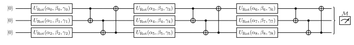
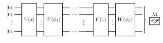
We now evaluate our theoretical findings based on a 2D classification problem, which we call the circle classification problem [52]: within a domain of $𝒳=[-1,+1]\times [-1,+1]$, a circle with radius $\sqrt{2/\pi }$ is drawn, and all data points inside the circle are labeled with $y=+1$, whereas points outside are labeled with $y=-1$, see Figure 6 in the Supplementary Section 3. For the quantum model with trainable encoding, we use general SU(2) operators and encode $w_j^{\top }x+{\theta }_j$ into the first two rotation angles. We repeat this encoding for each of the considered $3$ qubits, followed by nearest neighbour entangling gates based on CNOTs. Such a layer is then repeated $3$ times. As observable, we use $ℳ=Z\otimes Z\otimes Z$. The resulting circuit is illustrated in Figure 4.

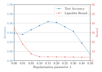
The numerical results for the robustness simulations are shown in Figure 2, where we compare the worst-case test accuracy and Lipschitz bound of three trained models with different regularization parameter $\lambda \in \{0,0.2,0.5\}$. Additionally, the plot shows the accuracy of a quantum model with fixed encoding for the same numbers of qubits and layers (see (16) and Supplementary Section 3 for details). The worst-case test accuracy of all models is obtained by sampling different noise samples $\epsilon$ from $[-\overline{\epsilon },+\overline{\epsilon }]$ and, thereby, it approximates the accuracy resulting from an adversarial attack norm-bounded by $\overline{\epsilon }$. As expected, all four models deteriorate with increasing noise level. For zero noise level $\overline{\epsilon }=0$, the model with the largest regularization parameter $\lambda =0.5$ (and, hence, the smallest Lipschitz bound $L_{\mathrm{\Theta }}=3.66$) has a smaller test accuracy than the non-regularized model with $\lambda =0$. This can be explained by a decrease in the training accuracy that is caused via the additional regularization in the cost. For increasing noise levels, however, the enhanced robustness outweighs the loss of training performance and, therefore, the model with $\lambda =0.5$ outperforms the model with $\lambda =0$. The fixed-encoding model achieves comparable performance to the trainable-encoding model with $\lambda =0.5$ for small noise and the worst performance among all models for high noise. These observations can be explained by the reduced expressivity yet high Lipschitz bound of the fixed-encoding model. Finally, the model with $\lambda =0.2$ almost consistently outperforms the model with $\lambda =0$ and, in particular, it yields a higher test accuracy for small noise levels. This can be explained by the improved generalization performance caused by the regularization, an effect we discuss in more detail in the following.

Generalization of quantum models. The Lipschitz bound (5) not only influences robustness but also has a crucial impact on generalization properties of the quantum model $f_{\mathrm{\Theta }}$. Intuitively, a smaller Lipschitz bound implies a smaller variability of $f_{\mathrm{\Theta }}$ and, therefore, reduces the risk of overfitting. This intuition is made formal via the following generalization bound.

Figure 3: Results for the generalization simulations for the circle classification problem. The training setup is identical to the robustness simulations as described in Figure 2. As test set, we draw $10.000$ points uniformly at random and evaluate the trained models with different regularization parameter $\lambda$. We plot the dependency of the test accuracy and the Lipschitz bound on the hyperparameter $\lambda$.

Figure 4: The trainable encoding quantum model employed in our numerical case studies uses general $U_{\mathrm{Rot}}\in \mathrm{SU}(2)$ unitaries parametrized by three Euler angles ${\alpha }_i$, ${\beta }_i$, ${\gamma }_i$, that each have the form $w_i^{\top }x+{\theta }_i$ for trainable parameters $w_i$, ${\theta }_i$. We set ${\gamma }_j=0$, $j=0,\mathrm{\dots },8$, to enable a fair comparison to a quantum model with fixed encoding (since the data are two-dimensional, only two angles are needed for encoding the data via the latter).

Theorem 1.

(informal version) Consider a supervised learning setup with loss $\mathrm{\ell }$ and data set $(x_k,y_k)\in 𝒳\times 𝒴$ of size $n$ drawn according to the probability distribution $P$. For the quantum model $f_{\mathrm{\Theta }}$ from (4), define the expected risk

$ℛ(f_{\mathrm{\Theta }})={\displaystyle {\int }_{𝒳\times 𝒴}}\mathrm{\ell }(y,f_{\mathrm{\Theta }}(x))dP(x,y)$ (10)

and the empirical risk

${ℛ}_n(f_{\mathrm{\Theta }})={\displaystyle \frac{1}{n}}{\displaystyle \sum _{k=1}^n}\mathrm{\ell }(y_k,f_{\mathrm{\Theta }}(x_k)).$ (11)

The generalization error of $f_{\mathrm{\Theta }}$ is bounded as

$\left|ℛ(f_{\mathrm{\Theta }})-{ℛ}_n(f_{\mathrm{\Theta }})\right|\le$ $C_1\parallel ℳ\parallel {\displaystyle \sum _{j=1}^N}\parallel w_j\parallel \parallel H_j\parallel +{\displaystyle \frac{C_2}{\sqrt{n}}}$ (12)

for some $C_1,C_2>0$.

The detailed version and proof of Theorem 1 are provided in Supplementary Section 2. Generalization bounds as in (12) quantify the ability of $f_{\mathrm{\Theta }}$ to generalize beyond the available data. The bound (12) directly depends on the data encoding via ${\sum }_{j=1}^N\parallel w_j\parallel \parallel H_j\parallel$ and on the observable via $\parallel ℳ\parallel$. In particular, $f_{\theta }$ achieves a small generalization error if its Lipschitz bound $L_{\mathrm{\Theta }}$ is small and the size $n$ of the data set is large. Note, however, the following fundamental trade-off: A too small Lipschitz bound $L_{\mathrm{\Theta }}$ may limit the expressivity of $f_{\mathrm{\Theta }}$ and, therefore, lead to a high empirical risk ${ℛ}_n(f_{\mathrm{\Theta }})$, in which case the generalization bound (12) is meaningless. In conclusion, Theorem 1 implies a small expected risk $ℛ(f_{\mathrm{\Theta }})$ if $n$ is large, $L_{\mathrm{\Theta }}$ is small, and $f_{\mathrm{\Theta }}$ has a small empirical risk ${ℛ}_n(f_{\mathrm{\Theta }})$. In contrast to existing generalization bounds [22, 44, 45, 46, 47], the bound (12) explicitly involves the Lipschitz bound (5), i.e., the norm of the data encoding.

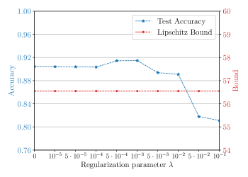
We evaluate the generalization performance of the trainable encoding again on the circle classification problem. The training setup is identical to the robustness simulations and the numerical results are shown in Figure 3, where we plot the test accuracy and Lipschitz bound depending on the regularization parameter $\lambda$. Increasing the regularization parameter $\lambda$ decreases the Lipschitz bound $L_{\mathrm{\Theta }}$ of the trained model. In accordance with the generalization bound (12), this reduction of $L_{\mathrm{\Theta }}$ improves generalization performance with the maximum test accuracy at $\lambda =0.15$. Beyond this value, the regularization causes a too small Lipschitz bound, limiting expressivity and, therefore, decreasing the training accuracy. As a result, the test accuracy decreases as well. This illustrates the role of $\lambda$ as a hyperparameter: Regularization does not always improve performance, but there is a sweet spot for $\lambda$ at which both superior generalization and robustness over the unregularized setup (i.e., $\lambda =0$) can be obtained. In practice, the hyperparameter $\lambda$ can be tuned, e.g., via cross-validation.

Benefits of trainable encodings. A popular class of quantum models is obtained by constructing circuits which alternate between data- and parameter-dependent gates, i.e., replacing $U_{\mathrm{\Theta }}(x)$ in (3) by

$U_{\phi }^{\mathrm{f}}(x)=W({\phi }_L)V(x)\mathrm{\cdots }W({\phi }_1)V(x),$ (13)

compare [49, 19, 20, 21, 22, 25]. The unitary operators $V,W$ are given by

$V(x)$ $=e^{-i{x}_D{G}_D}\mathrm{\cdots }{e}^{-i{x}_1{G}_1},$ (14)

$W({\phi }_j)$ $=e^{-i{\phi }_{j,p}{S}_p}\mathrm{\cdots }{e}^{-i{\phi }_{j,1}{S}_1}$ (15)

for trainable parameters ${\phi }_j$ and generators $G_i=G_i^{†}$, $S_i=S_i^{†}$. Figure 5 depicts the circuit representation of the corresponding quantum model

$f_{\phi }^{\mathrm{f}}(x)=⟨0|U_{\phi }^{\mathrm{f}}{(x)}^{†}ℳU_{\phi }^{\mathrm{f}}(x)|0⟩.$ (16)

Figure 5: Circuit representation of the quantum model (16) with fixed encoding.

It is not hard to show that the parametrized quantum circuit $U_{\mathrm{\Theta }}(x)$ in (3) generalizes the one in (13). Indeed, $U_{j,{\mathrm{\Theta }}_j}(x)$ in (2) reduces to either

$e^{-i{x}_j{G}_j}\text{or}{e}^{-i{\phi }_j{S}_j}$ (17)

for suitable choices of $w_j$, ${\theta }_j$, and $H_j$. Note that the data encoding of the quantum model $f_{\phi }^{\mathrm{f}}(x)$ is fixed a priori via the choice of $w_j$ and, in particular, it cannot be influenced during training. Therefore, we refer to $f_{\phi }^{\mathrm{f}}(x)$ as a quantum model with fixed encoding, in contrast to $f_{\mathrm{\Theta }}(x)$ in (4) which contains trainable parameters $w_j$ and, therefore, a trainable encoding.

Benefits of trainable encodings for the expressivity of quantum models have been demonstrated numerically in [53, 54, 55] and theoretically in [24, 25]. In the following, we discuss the importance of trainable encodings for robustness and generalization. Recall that the Lipschitz bound (5), which we showed to be a crucial quantifier of robustness and generalization of quantum models, only depends on the observable $ℳ$ and on the data encoding $w_j$, $H_j$, but it is independent of the parameters ${\theta }_j$. Hence, in the quantum model $f_{\phi }^{\mathrm{f}}(x)$ with fixed encoding, the Lipschitz bound (5) cannot be influenced during training and, instead, is fixed a priori via the choice of the Hermitian generators $G_j$. As a result, training has a limited effect on robustness and generalization properties of fixed-encoding quantum models.

The distinction between trainable and fixed data encodings becomes even more apparent when expressing quantum models as Fourier series [25]. In this case, fixed-encoding quantum models choose the frequencies of the Fourier basis functions before the training and only optimize over their coefficients. On the contrary, trainable-encoding quantum models simultaneously optimize over the frequencies and the coefficients which, according to the Lipschitz bound (5), is key for influencing robustness and generalization properties.

These insights confirm the observation by [56, 57, 58] that fixed-encoding quantum models are neither sensitive to data perturbations nor to overfitting. On the one hand, resilience against these two phenomena is a desirable property. However, the above discussion also implies that Lipschitz bound regularization, which is a systematic and effective tool for influencing robustness and generalization [2, 6, 16, 17, 18], cannot be implemented for fixed-encoding quantum models to improve robustness and generalization. The detrimental effect of this fact is illustrated by our robustness simulations in Figure 2. Here, the fixed-encoding model has a considerably higher Lipschitz bound than all the considered trainable-encoding models. This implies a significantly worse robustness w.r.t. data perturbations and, therefore, leads to a rapidly decreasing test accuracy for larger noise levels. Further, regularizing the parameters $\phi$ as suggested, e.g., by [59], does not affect the Lipschitz bound and, therefore, cannot be used to improve the robustness. In Supplementary Section 3, we study the effect of a regularization of $\phi$ on generalization. We find that the influence of regularizing the ${\phi }_j$’s on the test accuracy is limited and likely dependent on the specific ground-truth distribution generating the data and the chosen circuit ansatz.

To conclude, our results show that training the encoding in quantum models not only increases the expressivity but also leads to superior robustness and generalization properties.

Discussion

In this paper, we study robustness and generalization properties of quantum models based on Lipschitz bounds. Lipschitz bounds are a well-established tool in the classical ML literature which not only quantify adversarial robustness but are also closely connected to generalization performance. We derive Lipschitz bounds based on the size of the data encoding which we then use to study robustness and generalization properties. Given that our generalization bound explicitly involves the parameters of the data encoding, it is not a uniform bound. As a result, it may allow to overcome some of the limitations of uniform QML generalization bounds [48]. Further, our theoretical results highlight the role of trainable encodings combined with regularization techniques for obtaining robust and generalizable quantum models. The numerical results confirm our theoretical findings, showing the existence of a sweet spot for the regularization parameter for which our training scheme improves both robustness as well as generalization compared to a non-regularized training scheme. It is important to emphasize that these numerical results with specific choices of rotation and entangling gates are mainly used for illustration, but our theoretical framework applies to all quantum models that can be written as in (4) and, hence, also allow for different rotation gates, entangling layers, or even parametrized multi-qubit gates.

While our results indicate the potential of using Lipschitz bounds in QML, there are various promising directions for future research. First and foremost, transferring existing research on Lipschitz bounds in classical ML to the QML setting provides a systematic framework for handling robustness and generalization, beyond the first results presented in this paper. In particular, although we focus on variational quantum models, the basic principles of our results are transferrable to different quantum models, including quantum kernel methods [20, 21] or linear quantum models [23]. Further, while we have emphasized the importance of trainable encodings, the considered quantum model only employs a specific, affine encoding $w_j^{\top }x+{\theta }_j$. Extending our results to more general, possibly nonlinear encodings provides a promising avenue for designing powerful quantum models. Classical neural networks are ideal candidates for realizing a nonlinear encoding, given the extensive research in classical ML on their Lipschitz properties [2, 6, 9, 10, 11, 12, 13, 14, 15]. Finally, we plan to validate our theoretical findings for more complex classification tasks and on real quantum hardware.

Code Availability

The source code for the numerical case studies, as well as the data generation and analysis scripts are publicly accessible on GitHub via https://github.com/daniel-fink-de/training-robust-and-generalizable-quantum-models.

Supplementary material

1 Lipschitz bounds of quantum models

In this section, we study Lipschitz bounds of quantum models as in (4). We first derive a Lipschitz bound which is less tight than (5) but can be shown using a simple concatenation argument (Section 1-A). Next, in Section 1-B, we prove that (5) is indeed a Lipschitz bound.

1-A Simple Lipschitz bound based on concatenation

Before stating the result, we introduce the notation

$W=\left(\begin{array}{c}{w}_1^{\top }\\ \mathrm{⋮}\\ w_N^{\top }\end{array}\right),\mathrm{\Omega }=\left(\begin{array}{c}{\theta }_1\\ \mathrm{⋮}\\ {\theta }_N\end{array}\right).$ (18)

Theorem 2.

The following is a Lipschitz bound of $f_{\mathrm{\Theta }}$:

$L=2\parallel ℳ\parallel \parallel W\parallel {\displaystyle \sum _{j=1}^N}\parallel H_j\parallel .$ (19)

Proof.

Our proof relies on the fact that a Lipschitz bound of a concatenated function can be obtained based on the product of the individual Lipschitz bounds. To be precise, suppose $f$ can be written as $f=f_1\circ f_2\circ \mathrm{\cdots }\circ f_h$, where $\circ$ denotes concatenation and each $f_i$ admits a Lipschitz bound $L_i$, $i=1,\mathrm{\dots },h$. Then, for arbitrary input arguments $x,y$ of $f$, we obtain

$\parallel f(x)-f(y)\parallel$ $\le L_1\parallel f_2\circ \mathrm{\cdots }\circ f_h(x)-f_2\circ \mathrm{\cdots }\circ f_h(y)\parallel$

$\le \mathrm{\cdots }\le L_1{L}_2\mathrm{\cdots }{L}_h\parallel x-y\parallel .$ (20)

We now prove that (19) is a Lipschitz bound by representing $f_{\mathrm{\Theta }}$ as a concatenation of the three functions

$g_{\mathrm{meas}}(z_{\mathrm{m}})$ $=⟨z_{\mathrm{m}}|ℳ|z_{\mathrm{m}}⟩,$ (21)

$g_{\mathrm{unitary}}(z_{\mathrm{u}})$ $=e^{-i{z}_{\mathrm{u},N}{H}_N}\mathrm{\cdots }{e}^{-i{z}_{\mathrm{u},1}{H}_1}|0⟩,$ (22)

$g_{\mathrm{affine}}(z_{\mathrm{a}})$ $=W{z}_{\mathrm{a}}+\mathrm{\Omega }.$ (23)

More precisely, it holds that

$f_{\mathrm{\Theta }}(x)=g_{\mathrm{meas}}\circ g_{\mathrm{unitary}}\circ g_{\mathrm{affine}}(x).$ (24)

Hence, any set of Lipschitz bounds $L_{\mathrm{meas}}$, $L_{\mathrm{unitary}}$, $L_{\mathrm{affine}}$ for the three functions $g_{\mathrm{meas}}$, $g_{\mathrm{unitary}}$, $g_{\mathrm{affine}}$ gives rise to a Lipschitz bound of $f_{\mathrm{\Theta }}$ as their product:

$L=L_{\mathrm{meas}}{L}_{\mathrm{unitary}}{L}_{\mathrm{affine}}.$ (25)

Therefore, in the following, we will derive individual Lipschitz bounds $L_{\mathrm{meas}}$, $L_{\mathrm{unitary}}$, and $L_{\mathrm{affine}}$.
Lipschitz bound of $g_{\mathrm{meas}}$: Note that

${\displaystyle \frac{\mathrm{d}{g}_{\mathrm{meas}}(z_{\mathrm{m}})}{\mathrm{d}{z}_{\mathrm{m}}}}=2⟨z_{\mathrm{m}}|ℳ.$ (26)

Using $\parallel z_{\mathrm{m}}\parallel =1$, we infer

$\parallel {\displaystyle \frac{\mathrm{d}{g}_{\mathrm{meas}}(z_{\mathrm{m}})}{\mathrm{d}{z}_{\mathrm{m}}}}\parallel \le 2\parallel ℳ\parallel .$ (27)

Thus, $L_{\mathrm{meas}}=2\parallel ℳ\parallel$ is a Lipschitz bound of $g_{\mathrm{meas}}$.
Lipschitz bound of $g_{\mathrm{unitary}}$: It follows from [29, Theorem 2.2] that $L_{\mathrm{unitary}}={\sum }_{j=1}^N\parallel H_j\parallel$ is a Lipschitz bound of $g_{\mathrm{unitary}}$.
Lipschitz bound of $g_{\mathrm{affine}}$: Given the linear form of $g_{\mathrm{affine}}$, we directly obtain that $L_{\mathrm{affine}}=\parallel W\parallel$ is a Lipschitz bound. ∎

1-B Proof that (5) is a Lipschitz bound

We first derive a Lipschitz bound on the parametrized unitary $U_{\mathrm{\Theta }}(x)$. To this end, we compute its differential

$\mathrm{d}{U}_{\mathrm{\Theta }}(x)=$ $(\mathrm{d}{U}_{N,{\mathrm{\Theta }}_N}(x))U_{N-1,{\mathrm{\Theta }}_{N-1}}(x)\mathrm{\cdots }{U}_{1,{\mathrm{\Theta }}_1}(x)$ (28)

$+\mathrm{\cdots }+U_{N,{\mathrm{\Theta }}_N}(x)\mathrm{\cdots }{U}_{2,{\mathrm{\Theta }}_2}(x)(\mathrm{d}{U}_{1,{\mathrm{\Theta }}_1}(x))$

Note that each term $U_{j,{\mathrm{\Theta }}_j}(x)$ can be written as the concatenation of the two maps $g_j$ and $h_j$ defined by

$g_j(x)$ $=w_j^{\top }x+{\theta }_j$ (29)

$h_j(z_j)$ $=e^{-i{z}_j{H}_j}.$ (30)

To be precise, it holds that $U_{j,{\mathrm{\Theta }}_j}(x)=h_j\circ g_j(x)$. The differentials of the two maps $g_j$ and $h_j$ are given by

$\mathrm{d}{h}_j(z_j)(u)$ $=-i{H}_j{e}^{-i{z}_j{H}_j}u,$ (31)

$\mathrm{d}{g}_j(x)(v)$ $=w_j^{\top }v,$

where $h_j(z_j)(u)$ denotes the differential of $h_j$ at $z_j$ applied to $u\in ℝ$, and similarly for $g_j(x)(v)$. Thus, we have

$\mathrm{d}{U}_{j,{\mathrm{\Theta }}_j}(x)(v)$ $=(\mathrm{d}{h}_j(g_j(x)))\circ (\mathrm{d}{g}_j(x)(v))$ (32)

$=-i{H}_j{e}^{-i(w_j^{\top }x+{\theta }_j)H_j}{w}_j^{\top }v$

$=-i{H}_j{U}_{j,{\mathrm{\Theta }}_j}(x)w_j^{\top }v.$

Inserting this into (28), we obtain

$\mathrm{d}{U}_{\mathrm{\Theta }}(x)(v)=-i\left(H_N{U}_{\mathrm{\Theta }}(x)w_N^{\top }v+\mathrm{\cdots }+U_{\mathrm{\Theta }}(x)H_1{w}_1^{\top }v\right).$ (33)

We have thus shown that the Jacobian $J_{\mathrm{\Theta }}(x)$ of the map $U_{\mathrm{\Theta }}(x)|0⟩$ is given by

$J_{\mathrm{\Theta }}(x)=-i\left(H_N{U}_{\mathrm{\Theta }}(x)|0⟩w_N^{\top }+\mathrm{\cdots }+U_{\mathrm{\Theta }}(x)H_1|0⟩w_1^{\top }\right).$ (34)

Using that $|0⟩$ has unit norm, that the $U_{j,{\mathrm{\Theta }}_j}$’s are unitary, as well as the triangle inequality, the norm of $J_{\mathrm{\Theta }}(x)$ is bounded as

$\parallel J_{\mathrm{\Theta }}(x)\parallel \le {\displaystyle \sum _{j=1}^N}\parallel w_j\parallel \parallel H_j\parallel .$ (35)

Thus, ${\sum }_{j=1}^N\parallel w_j\parallel \parallel H_j\parallel$ is a Lipschitz bound of $U_{\mathrm{\Theta }}(x)|0⟩$ [60, p. 356].

Finally, $f_{\mathrm{\Theta }}(x)$ is a concatenation of $U_{\mathrm{\Theta }}(x)|0⟩$ and the function $z\mapsto ⟨z|ℳ|z⟩$, which admits the Lipschitz bound $2\parallel ℳ\parallel$, compare (27). Hence, a Lipschitz bound of $f_{\mathrm{\Theta }}$ can be obtained as the product of these two individual bounds, i.e., as in (5). ∎

2 Full version and proof of Theorem 1

We first state the main result in a general supervised learning setup, before applying it to the quantum model considered in this paper. Consider a supervised learning setup with data samples ${\{x_k,y_k\}}_{k=1}^n$ drawn independently and identically distributed from $𝒵≔𝒳\times 𝒴\subseteq {ℝ}^d\times ℝ$ according to some probability distribution $P$. We define the $ϵ$-covering number of $𝒵$ as follows.

Definition 2.1.

(adapted from [7, Definition 1]) We say that $\widehat{𝒵}$ is an $ϵ$-cover of $𝒵$, if, for all $z\in 𝒵$, there exists $\widehat{z}\in \widehat{𝒵}$ such that $\parallel z-\widehat{z}\parallel \le ϵ$. The $ϵ$-covering number of $𝒵$ is

$𝒩(ϵ,𝒵)=\min \{|\widehat{𝒵}|\mid \widehat{𝒵}\text{is an}ϵ\text{-cover of}𝒵\}.$ (36)

For a generic model $f:𝒳\to 𝒴$, a loss function $\mathrm{\ell }:𝒴\times 𝒴\to ℝ$, and the training data ${\{x_k,y_k\}}_{k=1}^n$, we define the expected loss and the empirical loss by

$ℛ(f)={\displaystyle {\int }_{𝒳\times 𝒴}}\mathrm{\ell }(y,f(x))dP(x,y)$ (37)

and

${ℛ}_n(f)={\displaystyle \frac{1}{n}}{\displaystyle \sum _{k=1}^n}\mathrm{\ell }(y_k,f(x_k)),$ (38)

respectively. The following result states a generalization bound of $f$.

Lemma 2.1.

Suppose

1. the loss $\mathrm{\ell }$ is nonnegative and admits a Lipschitz bound $L_{\mathrm{\ell }}>0$,

2. $𝒵$ is compact such that $M≔{sup}_{y,y^{\prime }\in 𝒴}\mathrm{\ell }(y,y^{\prime })$ is finite, and

3. $L_f>0$ is a Lipschitz bound of $f$.

Then, for any $\gamma ,\delta >0$, with probability at least $1-\delta$ the generalization error of $f$ is bounded as

$|ℛ(f)-{ℛ}_n(f)|$ (39)

$\le$ $\gamma L_{\mathrm{\ell }}\max \{1,L_f\}+M\sqrt{{\displaystyle \frac{2𝒩(\frac{\gamma }{2},𝒵)\ln 2+2\ln (\frac{1}{\delta })}{n}}}.$

Proof.

For the following proof, we invoke the concept of $(K,ϵ)$-robustness (adapted from [7, Definition 2]): The classifier $f$ is $(K,ϵ)$-robust for $K\in \mathbb{N}$ and $ϵ\in ℝ$, if $𝒵$ can be partitioned into $K$ disjoint sets, denoted by ${\{C_i\}}_{i=1}^K$, such that the following holds: For all $k=1,\mathrm{\dots },n$, $(x,y)\in 𝒵$, $i=1,\mathrm{\dots },K$, if $(x_k,y_k),(x,y)\in C_i$, then

$|\mathrm{\ell }(y_k,f(x_k))-\mathrm{\ell }(y,f(x))|\le ϵ.$ (40)

This property quantifies robustness of $f$ in the following sense: The set $𝒵$ can be partitioned into a number of subsets such that, if a newly drawn sample $(x,y)$ lies in the same subset as a testing sample $(x_k,y_k)$, then their associated loss values are close. Let us now proceed by noting that, for any $(x_k,y_k)$, $k=1,\mathrm{\dots },n$, and $(x,y)\in 𝒵$, it holds that

$|\mathrm{\ell }(y_k,f(x_k))-\mathrm{\ell }(y,f(x))|$ (41)

$\le$ $L_{\mathrm{\ell }}\parallel (y_k,f(x_k))-(y,f(x)){\parallel }_2$

$\le$ $L_{\mathrm{\ell }}\left(\parallel y_k-y\parallel +\parallel f(x_k)-f(x)\parallel \right)$

$\le$ $L_{\mathrm{\ell }}\max \{1,L_f\}\parallel (x_k,y_k)-(x,y)\parallel ,$

where we use the Lipschitz bound $L_{\mathrm{\ell }}$ of $\mathrm{\ell }$, the triangle inequality, and the Lipschitz bound $L_f$ of $f$, respectively. Using [7, Theorem 6], we infer that $f$ is $(𝒩(\frac{\gamma }{2},𝒵),L_{\mathrm{\ell }}\max \{1,L_f\}\gamma )$-robust for all $\gamma >0$. It now follows from [7, Theorem 1] that, for any $\delta >0$, with probability at least $1-\delta$ inequality (39) holds. ∎

Let us now combine the Lipschitz bound (5) and Lemma 2.1 to state a tailored generalization bound for the considered class of quantum models $f_{\mathrm{\Theta }}$, thus proving Theorem 1.

Theorem 2.1.

Suppose

1. the loss $\mathrm{\ell }$ is nonnegative and admits a Lipschitz bound $L_{\mathrm{\ell }}>0$ and

2. $𝒵$ is compact such that $M≔{sup}_{y,y^{\prime }\in 𝒴}\mathrm{\ell }(y,y^{\prime })$ is finite.

Then, for any $\gamma ,\delta >0$, with probability at least $1-\delta$ the generalization error of $f_{\mathrm{\Theta }}$ is bounded as

$|ℛ(f)-{ℛ}_n(f)|\le$ $\gamma L_{\mathrm{\ell }}\max \{1,2\parallel ℳ\parallel {\displaystyle \sum _{j=1}^N}\parallel w_j\parallel \parallel H_j\parallel \}$

$+M\sqrt{{\displaystyle \frac{2𝒩(\frac{\gamma }{2},𝒵)\ln 2+2\ln (\frac{1}{\delta })}{n}}}.$ (42)

Theorem 2.1 shows that the size of the data encoding and of the observable directly influences the generalization performance of the quantum model $f_{\mathrm{\Theta }}$. In particular, for smaller values of ${\sum }_{j=1}^N\parallel w_j\parallel \parallel H_j\parallel$ and $\parallel ℳ\parallel$, the expected loss is closer to the empirical loss. The right-hand side of (42) contains two terms: The first one depends on the parameters of the quantum model $f_{\mathrm{\Theta }}$ and characterizes its robustness via the Lipschitz bound (5), whereas the second term decays with increasing data length $n$. While (39) holds for arbitrary values of $\gamma >0$, it is not immediate which value of $\gamma$ leads to the smallest possible bound: Smaller values of $\gamma$ decrease the first term but increase $𝒩(\frac{\gamma }{2},𝒵)$ in the second term (and vice versa).

In contrast to existing QML generalization bounds [22, 44, 45, 46, 47], Theorem 2.1 explicitly highlights the role of the Lipschitz bound. Using the additional flexibility of the parameter $\gamma$, it can be shown that the generalization bound (42) converges to zero when the data length $n$ approaches infinity. To this end, we use [61, Lemma 6.27] to upper bound the covering number

$𝒩({\displaystyle \frac{\gamma }{2}},𝒵)\le {\left({\displaystyle \frac{6R}{\gamma }}\right)}^{D+1},$ (43)

where $R$ is the radius of the smallest ball containing $𝒵$. Inserting (43) into (42) and choosing $\gamma$ depending on $n$ as $\gamma =n^{-\frac{1}{2D+2}}$, we infer

$|ℛ(f)-{ℛ}_n(f)|\le$ ${\displaystyle \frac{1}{n^{\frac{1}{2D+2}}}}{L}_{\mathrm{\ell }}\max \{1,2\parallel ℳ\parallel {\displaystyle \sum _{j=1}^N}\parallel w_j\parallel \parallel H_j\parallel \}$

$+M\sqrt{{\displaystyle \frac{2\ln 2{\left(6R\right)}^{D+1}}{\sqrt{n}}}+{\displaystyle \frac{2\ln (\frac{1}{\delta })}{n}}},$ (44)

which indeed converges to zero for $n\to \mathrm{\infty }$.

3 Numerics: setup and further results

In the following, we provide details regarding the setup of our numerical results (Section 3-A) and we present further numerical results regarding parameter regularization in quantum models with fixed encoding (Section 3-B).

3-A Numerical setup

Figure 6: From left to right: Illustration of the ground truth of the circle classification problem, the decision boundary of the best trained model without regularization and the decision boundary with the best model for $\lambda =0.2$. The use of a regularization parameter during training shows a more regular decision boundary after the training.

All numerical simulations within this work were performed using the Python QML library PennyLane [62]. As device, we used the noiseless simulator ”lightning.qubit” together with the adjoint differentiation method, to enable fast and memory efficient gradient computations. In order to solve the optimization problem in (9), we apply the ADAM optimizer using a learning rate of $\eta =0.1$ and the suggested values for all other hyperparameters [63]. Furthermore, we run $200$ epochs throughout and train $9$ models based on different initial parameters for varying regularization parameters $\lambda >0$. Adding the regularization does not introduce significant computational overhead as the evaluation of the cost only involves a weighted sum of the terms ${\Vert w_j\Vert }^2$. As final model, we take the set of parameters for the model with minimal cost over all runs and epochs. Furthermore, the training as well as the robustness and generalization analysis were parallelized using Dask [64].

For the trainable encoding model, the classical data is encoded into the quantum circuit with a general $U_{\mathrm{Rot}}\in \mathrm{SU}(2)$ unitary parametrized by 3 Euler angles $U_{\mathrm{Rot}}({\alpha }_j,{\beta }_j,{\gamma }_j)$ with

${\alpha }_j$ $=w_{j,1}^{\top }x+{\theta }_{j,1},$ (45)

${\beta }_j$ $=w_{j,2}^{\top }x+{\theta }_{j,2},$ (46)

${\gamma }_j$ $=w_{j,3}^{\top }x+{\theta }_{j,3}.$ (47)

$U_{\mathrm{Rot}}$ in PennyLane is implemented by the following decomposition

$U_{\mathrm{Rot}}(\alpha ,\beta ,\gamma )$ $=R_Z(\gamma )R_Y(\beta )R_Z(\alpha ),$ (48)

(49)

Figure 7: Results for the generalization simulations for the circle classification problem when using the fixed-encoding quantum model (16) and regularization of the parameters $\phi$. The training and test setup are identical to simulations shown in Figures 2 and 3. We plot the dependency of the test accuracy and the Lipschitz bound on the hyperparameter $\lambda$ entering the regularized training problem (50).

In our numerical case study we set ${\gamma }_j=0$ for all $j$ since this 1) still allows to reach arbitrary points on the Bloch sphere and 2) enables an easier comparison to fixed-encoding quantum models. In order to introduce entanglement in a hardware-efficient way, we use a ring of CNOTs. The considered circuit shown in Figure 4 involves three layers of rotations and entanglement, which we observed to be a good trade-off between expressivity and generalization. More precisely, in our simulations, fewer layers were not sufficient to accurately solve the classification task, whereas more layers led to higher degrees of overfitting. For the fixed-encoding quantum models as in (16), we use a similar $3$-layer ansatz, encoding the two entries of the 2D data points into the first and second angle ${\alpha }_j$, ${\beta }_j$ of the rotation gates, followed by a parametrized $\mathrm{SU}(2)$ rotation with three free parameters. We also perform a classical data pre processing, scaling the input domain from $[-1,+1]$ to $[-\pi ,+\pi ]$, such that the full possible range of the rotation angles can be utilized.

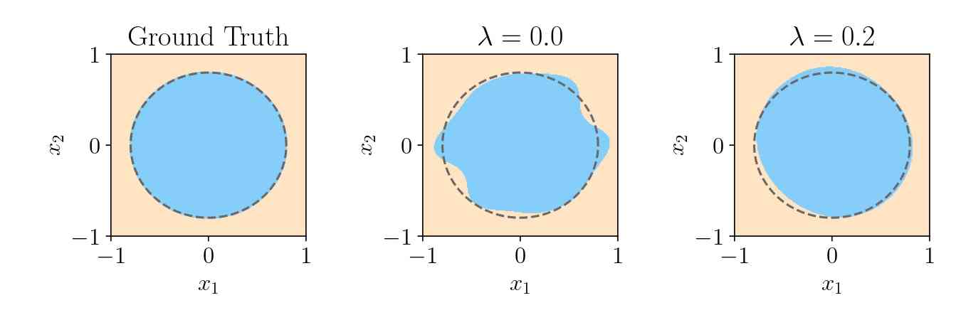
In Figure 6, we plot the ground truth and the decision boundaries for the two quantum models corresponding to $\lambda =0.0$ and $\lambda =0.2$. As expected, the decision boundary resulting from the regularized training is significantly smoother than the unregularized one, explaining the superior robustness and generalization of the former.

3-B Regularization in quantum models with fixed encoding

In the main text, we have seen that the Lipschitz bound of the quantum model with fixed encoding $f_{\phi }^{\mathrm{f}}(x)$ in (16) cannot be adapted by changing the parameters $\phi$. As a result, it is not possible to use Lipschitz bound regularization for improving robustness and generalization. In the following, we investigate whether regularization of $\phi$ can instead be used to improve generalization performance. More precisely, we consider the same numerical setup as for our generalization results with trainable encoding depicted in Figure 3. The main difference is that we consider a fixed-encoding quantum model $f_{\phi }^{\mathrm{f}}(x)$ which is trained via the following regularized training problem

$\underset{\phi }{\min }{\displaystyle \frac{1}{n}}{\displaystyle \sum _{k=1}^n}\mathrm{\ell }(f_{\phi }^{\mathrm{f}}(x_k),y_k)+\lambda {\displaystyle \sum _{j=1}^L}{\parallel {\phi }_j\parallel }^2.$ (50)

The regularization with hyperparameter $\lambda >0$ aims at keeping the norms of the angles ${\phi }_j$ small. Figure 7 depicts the test accuracy and Lipschitz bound of the resulting quantum model for different regularization parameters $\lambda$. First, note that the Lipschitz bound is indeed constant for all choices of $\lambda$ due to the fixed encoding. Comparing Figures 3 and 7, we see that the trainable encoding yields a significantly higher test accuracy in comparison to the fixed encoding. Moreover, the influence of the regularization parameter on the test accuracy is much less pronounced for the fixed encoding than for the trainable encoding, confirming our previous discussion on the benefits of trainable encodings. The test accuracy is not entirely independent of $\lambda$ since 1) regularization of the parameters ${\phi }_j$ influences the optimization and can improve or deteriorate convergence and 2) biasing $\phi$ towards zero may be beneficial if the underlying ground-truth distribution is better approximated by a quantum model with small values $\phi$. Whether 2) brings practical benefits is, however, highly problem-specific as it depends on the distribution generating the data and on the circuit ansatz.

References

- [1] I. J. Goodfellow, J. Shlens, and C. Szegedy, “Explaining and harnessing adversarial examples,” arXiv:1412.6572, 2014.
- [2] C. Szegedy, W. Zaremba, I. Sutskever, J. Bruna, D. Erhan, I. Goodfellow, and R. Fergus, “Intriguing properties of neural networks,” arXiv:1312.6199, 2014.
- [3] E. Wong and Z. Kolter, “Provable defenses against adversarial examples via the convex outer adversarial polytope,” in Proc. International Conference on Machine Learning, 2018, pp. 5283–5292.
- [4] Y. Tsuzuku, I. Sato, and M. Sugiyama, “Lipschitz-margin training: Scalable certification of perturbation invariance for deep neural networks,” in Proc. Advances in Neural Information Processing Systems, 2018, pp. 6541–6550.
- [5] A. Madry, A. Makelov, L. Schmidt, D. Tsipras, and A. Vladu, “Towards deep learning models resistant to adversarial attacks,” arXiv:1706.06083, 2019.
- [6] A. Krogh and J. Hertz, “A simple weight decay can improve generalization,” in Advances in Neural Information Processing Systems, vol. 4, 1991. [Online]. Available: https://proceedings.neurips.cc/paper/1991/file/8eefcfdf5990e441f0fb6f3fad709e21-Paper.pdf
- [7] H. Xu and S. Mannor, “Robustness and generalization,” Mach. Learn., vol. 86, no. 3, pp. 391–423, 2012.
- [8] N. Papernot, P. McDaniel, X. Wu, S. Jha, and A. Swami, “Distillation as a defense to adversarial perturbations against deep neural networks,” in Proc. IEEE Symposium on Security and Privacy (SP), 2016, pp. 582–597.
- [9] U. von Luxburg and O. Bousquet, “Distance-based classification with Lipschitz functions,” Journal of Machine Learning Research, vol. 5, pp. 669–695, 2004.
- [10] P. Bartlett, D. J. Foster, and M. Telgarsky, “Spectrally-normalized margin bounds for neural networks,” in Advances in Neural Information Processing Systems, vol. 30, 2017, pp. 6240–6249.
- [11] B. Neyshabur, S. Bhojanapalli, D. McAllester, and N. Srebro, “Exploring generalization in deep learning,” in Advances in Neural Information Processing Systems, 2017, pp. 5947–5956.
- [12] J. Sokolić, R. Giryes, G. Sapiro, and M. R. D. Rodrigues, “Robust large margin deep neural networks,” IEEE Trans. Signal Processing, vol. 65, no. 16, pp. 4265–4280, 2017.
- [13] T.-W. Weng, H. Zhang, P.-Y. Chen, J. Yi, D. Su, Y. Gao, C.-J. Hsieh, and L. Daniel, “Evaluating the robustness of neural networks: an extreme value theory approach,” in Proc. 6th Int. Conf. Learning Representations (ICLR), 2018.
- [14] W. Ruan, X. Huang, and M. Kwiatkowska, “Reachability analysis of deep neural networks with provable guarantees,” in Proc. 27th Int. joint Conf. Artificial Intelligence (IJCAI), 2018, pp. 2651–2659.
- [15] C. Wei and T. Ma, “Data-dependent sample complexity of deep neural networks via Lipschitz augmentation,” in Advances in Neural Information Processing Systems, 2019, pp. 9725–9736.
- [16] M. Hein and M. Andriushchenko, “Formal guarantees on the robustness of a classifier against adversarial manipulation,” in Proc. Advances in Neural Information Processing Systems, 2017, pp. 2266–2276.
- [17] H. Gouk, E. Frank, B. Pfahringer, and M. Cree, “Regularisation of neural networks by enforcing Lipschitz continuity,” Machine Learning, vol. 110, pp. 393–416, 2021.
- [18] P. Pauli, A. Koch, J. Berberich, P. Kohler, and F. Allgöwer, “Training robust neural networks using Lipschitz bounds,” IEEE Control Systems Lett., vol. 6, pp. 121–126, 2022.
- [19] M. Benedetti, E. Lloyd, S. Sack, and M. Fiorentini, “Parameterized quantum circuits as machine learning models,” Quantum Sci. Technol., vol. 4, p. 043001, 2019.
- [20] V. Havlíček, A. D. Córcoles, K. Temme, A. W. Harrow, A. Kandala, J. M. Chow, and J. M. Gambetta, “Supervised learning with quantum-enhanced feature spaces,” Nature, vol. 567, pp. 209–212, 2019.
- [21] M. Schuld and N. Killoran, “Quantum machine learning in feature Hilbert spaces,” Physical Review Letters, vol. 122, p. 040504, 2019.
- [22] A. Abbas, D. Sutter, C. Zoufal, A. Lucchi, A. Figalli, and S. Woerner, “The power of quantum neural networks,” Nature Computational Science, vol. 1, pp. 403–409, 2021.
- [23] S. Jerbi, L. J. Fiderer, H. P. Nautrup, J. M. Kübler, H. J. Briegel, and V. Dunjko, “Quantum machine learning beyond kernel methods,” Nature Communications, vol. 14, p. 517, 2023.
- [24] A. Pérez-Salinas, A. Cervera-Lierta, E. Gil-Fuster, and J. I. Latorre, “Data re-uploading for a universal quantum classifier,” Quantum, vol. 4, p. 226, 2020.
- [25] M. Schuld, R. Sweke, and J. J. Meyer, “Effect of data encoding on the expressive power of variational quantum-machine-learning models,” Physical Review A, vol. 103, p. 032430, 2021.
- [26] J. Preskill, “Quantum computing in the NISQ era and beyond,” Quantum, vol. 2, p. 79, 2018.
- [27] R. LaRose and B. Coyle, “Robust data encodings for quantum classifiers,” Physical Review A, vol. 102, p. 032420, 2020.
- [28] L. Cincio, K. Rudinger, M. Sarovar, and P. J. Coles, “Machine learning of noise-resilient quantum circuits,” PRX Quantum, vol. 2, p. 010324, 2021.
- [29] J. Berberich, D. Fink, and C. Holm, “Robustness of quantum algorithms against coherent control errors,” arXiv:2303.00618, 2023.
- [30] D. Edwards and D. B. Rawat, “Quantum adversarial machine learning: status, challenges and perspectives,” in Proc. 2nd IEEE Int. Conf. Trust, Privacy and Security in Intelligent Systems and Applications (TPS-ISA), 2020, pp. 128–133.
- [31] M. T. West, S.-L. Tsang, J. S. Low, C. D. Hill, C. Leckie, L. C. L. Hollenberg, S. M. Erfani, and M. Usman, “Towards quantum enhanced adversarial robustness in machine learning,” arXiv:2306.12688, 2023.
- [32] S. Lu, L.-M. Duan, and D.-L. Deng, “Quantum adversarial machine learning,” Physical Review Research, vol. 2, p. 033212, 2020.
- [33] M. T. West, S. M. Erfani, C. Leckie, M. Sevior, L. C. L. Hollenberg, and M. Usman, “Benchmarking adversarially robust quantum machine learning at scale,” arXiv:2211.12681, 2022.
- [34] N. Liu and P. Wittek, “Vulnerability of quantum classification to adversarial perturbations,” Physical Review A, vol. 101, p. 062331, 2020.
- [35] H. Liao, I. Convy, W. J. Huggins, and K. B. Whaley, “Robust in practice: adversarial attacks on quantum machine learning,” Physical Review A, vol. 103, p. 042427, 2021.
- [36] Y. Du, M.-H. Hsieh, T. Liu, D. Tao, and N. Liu, “Quantum noise protects quantum classifiers against adversaries,” Physical Review Research, vol. 3, p. 023153, 2021.
- [37] J. Guan, W. Fang, and M. Ying, “Robustness verification of quantum classifiers,” in Proc. Int. Conf. Computer Aided Verification, 2021, pp. 151–174.
- [38] M. Weber, N. Liu, B. Li, C. Zhang, and Z. Zhao, “Optimal provable robustness of quantum classification via quantum hypothesis testing,” Quantum Information, vol. 7, p. 76, 2021.
- [39] W. Gong and D.-L.-. Deng, “Universal adversarial examples and perturbations for quantum classifiers,” National Science Review, vol. 9, no. 6, p. nwab130, 2022.
- [40] W. Ren, W. Li, S. Xu, K. Wang, W. Jiang, F. Jin, X. Zhu, J. Chen, Z. Song, P. Zhang, H. Dong, X. Zhang, J. Deng, Y. Gao, C. Zhang, Y. Wu, B. Zhang, Q. Guo, H. Li, Z. Wang, J. Biamonte, C. Song, D.-L. Deng, and H. Wang, “Experimental quantum adversarial learning with programmable superconducting qubits,” arXiv:2204.01738, 2022.
- [41] H. Xiao, K. Rasul, and R. Vollgraf, “Fashion-MNIST: a novel image dataset for benchmarking machine learning algorithms,” arXiv:1708.07747, 2017.
- [42] M. Cerezo, G. Verdon, H.-Y. Huang, L. Cincio, and P. J. Coles, “Challenges and opportunities in quantum machine learning,” Nature Computational Science, vol. 2, pp. 567–576, 2022.
- [43] E. Peters and M. Schuld, “Generalization despite overfitting in quantum machine learning models,” arXiv:2209.05523, 2022.
- [44] H.-Y. Huang, M. Bourghton, M. Mohseni, R. Babbush, S. Boixo, H. Neven, and J. R. McClean, “Power of data in quantum machine learning,” Nature communications, vol. 12, no. 1, pp. 1–9, 2021.
- [45] L. Banchi, J. Pereira, and S. Pirandola, “Generalization in quantum machine learning: a quantum information standpoint,” PRX Quantum, vol. 2, p. 040321, 2021.
- [46] M. C. Caro, E. Gil-Fuster, J. J. Meyer, J. Eisert, and R. Sweke, “Encoding-dependent generalization bounds for parametrized quantum circuits,” arXiv:2106.03880, 2021.
- [47] S. Jerbi, C. Gyurik, S. C. Marshall, R. Molteni, and V. Dunjko, “Shadows of quantum machine learning,” arXiv:2306.00061, 2023.
- [48] E. Gil-Fuster, J. Eisert, and C. Bravo-Prieto, “Understanding quantum machine learning also requires rethinking generalization,” arXiv:2306.13461, 2023.
- [49] M. Schuld and F. Petruccione, Machine learning with quantum computers. Springer, 2021.
- [50] E. Farhi, J. Goldstone, and S. Gutmann, “A quantum approximate optimization algorithm,” arXiv:1411.4028, 2014.
- [51] S. Hadfield, Z. Wang, E. G. Rieffel, B. O’Gorman, D. Venturelli, and R. Biswas, “Quantum approximate optimization with hard and soft constraints,” in Proc. 2nd Int. Workshop on Post Moores Era Supercomputing, 2017, pp. 15–21.
- [52] S. Ahmed, “Tutorial: Data reuploading circuits,” https://pennylane.ai/qml/demos/tutorial˙data˙reuploading˙classifier/, 2021.
- [53] F. J. Gil Vidal and D. O. Theis, “Input redundancy for parameterized quantum circuits,” Frontiers in Physics, vol. 8, p. 297, 2020.
- [54] E. Ovalle-Magallanes, D. E. Alvarado-Carrillo, J. G. Avina-Cervantes, I. Cruz-Aceves, and J. Ruiz-Pinales, “Quantum angle encoding with learnable rotation applied to quantum-classical convolutional neural networks,” Applied Soft Computing, vol. 141, p. 110307, 2023.
- [55] B. Jaderberg, A. A. Gentile, Y. A. Berrada, E. Shishenina, and V. E. Elfving, “Let quantum neural networks choose their own frequencies,” arXiv:2309.03279, 2023.
- [56] K. Mitarai, M. Negoro, M. Kitagawa, and K. Fujii, “Quantum circuit learning,” Physical Review A, vol. 98, p. 032309, 2018.
- [57] M. Schuld, A. Bocharov, K. Svore, and N. Wiebe, “Circuit-centric quantum classifiers,” Physical Review A, vol. 101, p. 032308, 2020.
- [58] C.-C. Chen, M. Watabe, K. Shiba, M. Sogabe, K. Sakamoto, and T. Sogabe, “On the expressibility and overfitting of quantum circuit learning,” ACM Transactions on Quantum Computing, vol. 2, no. 2, p. 8, 2021.
- [59] Y. Du, M.-H. Hsieh, T. Liu, S. You, and D. Tao, “Learnability of quantum neural networks,” PRX Quantum, vol. 2, p. 040337, 2021.
- [60] T. M. Apostol, Mathematical Analysis. Pearson Education, 1974, 2nd edition.
- [61] M. Mohri, A. Rostamizadeh, and A. Talwalkar, Foundations of machine learning, 2nd ed., Adaptive Computation and Machine Learning. MIT Press, Cambridge, MA, 2018.
- [62] V. Bergholm, J. Izaac, M. Schuld, C. Gogolin, S. Ahmed, V. Ajith, M. S. Alam, G. Alonso-Linaje, B. AkashNarayanan, A. Asadi, J. M. Arrazola, U. Azad, S. Banning, C. Blank, T. R. Bromley, B. A. Cordier, J. Ceroni, A. Delgado, O. D. Matteo, A. Dusko, T. Garg, D. Guala, A. Hayes, R. Hill, A. Ijaz, T. Isacsson, D. Ittah, S. Jahangiri, P. Jain, E. Jiang, A. Khandelwal, K. Kottmann, R. A. Lang, C. Lee, T. Loke, A. Lowe, K. McKiernan, J. J. Meyer, J. A. Montañez-Barrera, R. Moyard, Z. Niu, L. J. O’Riordan, S. Oud, A. Panigrahi, C.-Y. Park, D. Polatajko, N. Quesada, C. Roberts, N. Sá, I. Schoch, B. Shi, S. Shu, S. Sim, A. Singh, I. Strandberg, J. Soni, A. Száva, S. Thabet, R. A. Vargas-Hernández, T. Vincent, N. Vitucci, M. Weber, D. Wierichs, R. Wiersema, M. Willmann, V. Wong, S. Zhang, and N. Killoran, “Pennylane: Automatic differentiation of hybrid quantum-classical computations,” arXiv:1811.04968, 2018.
- [63] D. P. Kingma and J. Ba, “Adam: a method for stochastic optimization,” arXiv:1412.6980, 2014.
- [64] Dask Development Team, “Dask: Library for dynamic task scheduling,” https://dask.org, 2016.