Are we really making much progress? Revisiting, benchmarking, and refining heterogeneous graph neural networks

Abstract.

Heterogeneous graph neural networks (HGNNs) have been blossoming in recent years, but the unique data processing and evaluation setups used by each work obstruct a full understanding of their advancements. In this work, we present a systematical reproduction of 12 recent HGNNs by using their official codes, datasets, settings, and hyperparameters, revealing surprising findings about the progress of HGNNs. We find that the simple homogeneous GNNs, e.g., GCN and GAT, are largely underestimated due to improper settings. GAT with proper inputs can generally match or outperform all existing HGNNs across various scenarios. To facilitate robust and reproducible HGNN research, we construct the Heterogeneous Graph Benchmark (HGB), consisting of 11 diverse datasets with three tasks. HGB standardizes the process of heterogeneous graph data splits, feature processing, and performance evaluation. Finally, we introduce a simple but very strong baseline Simple-HGN—which significantly outperforms all previous models on HGB—to accelerate the advancement of HGNNs in the future.

1. Introduction

As graph neural networks (GNNs) (Kipf and Welling, 2017; Battaglia et al., 2018) have already occupied the centre stage of graph mining research within recent years, the researchers begin to pay attention to their potential on heterogeneous graphs (a.k.a., Heterogeneous Information Networks) (Hu et al., 2020b; Dong et al., 2017; Wang et al., 2019b; Yun et al., 2019; Fu et al., 2020; Yang et al., 2020b). Heterogeneous graphs consist of multiple types of nodes and edges with different side information, connecting the novel and effective graph-learning algorithms to the noisy and complex industrial scenarios, e.g., recommendation.

To tackle the challenge of heterogeneity, various heterogeneous GNNs (HGNNs) (Wang et al., 2019b; Yun et al., 2019; Yang et al., 2020b) have been proposed to address the relevant tasks, including node classification, link prediction, and knowledge-aware recommendation. Take node classification for example, numerous HGNNs, such as HAN (Wang et al., 2019b), GTN (Yun et al., 2019), RSHN (Zhu et al., 2019), HetGNN (Zhang et al., 2019), MAGNN (Fu et al., 2020), HGT (Hu et al., 2020a), and HetSANN (Hong et al., 2020) were developed within the last two years.

Despite various new models developed, our understanding of how they actually make progress has been thus far limited by the unique data processing and settings adopted by each of them. To fully picture the advancements in this field, we comprehensively reproduce the experiments of 12 most popular HGNN models by using the codes, datasets, experimental settings, hyperparameters released by their original papers. Surprisingly, we find that the results generated by these state-of-the-art HGNNs are not as exciting as promised (Cf. Table 1), that is:

1. The performance of simple homogeneous GNNs, i.e., GCN (Kipf and Welling, 2017) and GAT (Veličković et al., 2017), is largely underestimated. Even vanilla GAT can outperform existing HGNNs in most cases with proper inputs.

2. Performances of some previous works are mistakenly reported due to inappropriate settings or data leakage.

Our further investigation also suggests:

1. Meta-paths are not necessary in most heterogeneous datasets.

2. There is still considerable room for improvements in HGNNs.

In our opinion, the above situation occurs largely because the individual data and experimental setup by each work obstructs a fair and consistent validation of different techniques, thus greatly hindering the advancements of HGNNs.

To facilitate robust and open HGNN developments, we build the Heterogeneous Graph Benchmark (HGB). HGB currently contains 11 heterogeneous graph datasets that vary in heterogeneity (the number of node and edge types), tasks (node classification, link prediction, and knowledge-aware recommendation), and domain (e.g., academic graphs, user-item graphs, and knowledge graphs). HGB provides a unified interface for data loading, feature processing, and evaluation, offering a convenient and consistent way to compare HGNN models. Similar to OGB (Hu et al., 2020c), HGB also hosts a leaderboard (https://www.biendata.xyz/hgb) for publicizing reproducible state-of-the-art HGNNs.

Finally, inspired by GAT’s significance in Table 1, we take GAT as backbone to design an extremely simple HGNN model—Simple-HGN. Simple-HGN can be viewed as GAT enhanced by three existing techniques: (1) learnable type embedding to leverage type information, (2) residual connections to enhance modeling power, and (3) $L_2$ normalization on the output embedddings. In ablation studies, these techniques steadily improve the performance. Experimental results on HGB suggest that Simple-HGN can consistently outperform previous HGNNs on three tasks across 11 datasets, making it to date the first HGNN model that is significantly better than the vanilla GAT.

To sum up, this work makes the following contributions:

• We revisit HGNNs and identify issues blocking progress;

• We benchmark HGNNs by HGB for robust developments;

• We refine HGNNs by designing the Simple-HGN model.

Table 1. Reproduction of Heterogeneous GNNs with simple GCN and GAT as baselines—all reproduction experiments use official codes and the same dataset, settings, hyperparameters as the original paper. The line with star (*) are results reported in the paper, and the lines without star are our reproduction. “-” means the results are not reported in the original paper. We mark the reproduction terms with $>$1 point gap compared to the reported results by $\mathbf{\uparrow }$ and $\mathbf{\downarrow }$. We also keep the standard variance terms above 1.

	HAN (Wang et al., 2019b)		GTN (Yun et al., 2019)			RSHN (Zhu et al., 2019)			HetGNN (Zhang et al., 2019)				MAGNN (Fu et al., 2020)
Dataset	ACM		DBLP	ACM	IMDB	AIFB	MUTAG	BGS	MC (10%)		MC (30%)		DBLP
Metric	Macro-F1	Micro-F1	Macro-F1	Macro-F1	Macro-F1	Accuracy	Accuracy	Accuracy	Macro-F1	Micro-F1	Macro-F1	Micro-F1	Macro-F1	Micro-F1
model*	91.89	91.85	94.18	92.68	60.92	97.22	82.35	93.10	97.8	97.9	98.1	98.2	93.13	93.61
GCN*	89.31	89.45	87.30	91.60	56.89	-	-	-	-	-	-	-	88.00	88.51
GAT*	90.55	90.55	93.71	92.33	58.14	91.67	72.06	66.32	96.2	96.3	96.5	96.5	91.05	91.61
model	90.94	90.96	92.95$\mathbf{\downarrow }$	92.28	57.53$\pm$2.22$\mathbf{\downarrow }$	97.22	82.35	93.10	97.06	97.11	97.34	97.37	92.81	93.36
GCN	92.25$\mathbf{\uparrow }$	92.29$\mathbf{\uparrow }$	91.48$\mathbf{\uparrow }$	92.28	59.11$\pm$1.73$\mathbf{\uparrow }$	97.22	79.41	96.55	91.88	92.04	95.37	95.57	88.31	89.37
GAT	92.08$\mathbf{\uparrow }$	92.15$\mathbf{\uparrow }$	94.18	92.49	58.86$\pm$1.73	100$\mathbf{\uparrow }$	80.88$\mathbf{\uparrow }$	100$\mathbf{\uparrow }$	98.25$\mathbf{\uparrow }$	98.30$\mathbf{\uparrow }$	98.42$\mathbf{\uparrow }$	98.50$\mathbf{\uparrow }$	94.40$\mathbf{\uparrow }$	94.78$\mathbf{\uparrow }$

2. Preliminaries

2.1. Heterogeneous Graph

A heterogeneous graph (Sun and Han, 2012) can be defined as $G=\{V,E,\varphi ,\psi \}$, where $V$ is the set of nodes and $E$ is the set of edges. Each node $v$ has a type $\varphi (v)$, and each edge $e$ has a type $\psi (e)$. The sets of possible node types and edge types are denoted by $T_v=\{\varphi (v):\forall v\in V\}$ and $T_e=\{\psi (e):\forall e\in E\}$, respectively. When $|T_v|=|T_e|=1$, the graph degenerates into an ordinary homogeneous graph.

2.2. Graph Neural Networks

GNNs aim to learn a representation vector ${𝒉}_v^{(L)}\in {ℝ}^{d_L}$ for each node $v$ after L-layer transformations, based on the graph structure and the initial node feature ${𝒉}_v^{(0)}\in {ℝ}^{d_0}$. The final representation can serve various downstream tasks, e.g., node classification, graph classification (after pooling), and link prediction.

Graph Convolution Network (GCN) (Kipf and Welling, 2017) is the pioneer of GNN models, where the $l^{th}$ layer is defined as

(1) $${𝑯}^{(l)}=\sigma (\widehat{𝑨}{𝑯}^{(l-1)}{𝑾}^{(l)}),$$

where ${𝑯}^{(l)}$ is the representation of all nodes after the $l^{th}$ layer. ${𝑾}^{(l)}$ is a trainable weight matrix. $\sigma$ is the activation function, and $\widehat{𝑨}$ is the normalized adjacency matrix with self-connections.

Graph Attention Network (GAT) (Veličković et al., 2017) later replaces the average aggregation from neighbors, i.e., $\widehat{𝑨}{𝑯}^{(l-1)}$, as a weighted one, where the weight ${\alpha }_{ij}$ for each edge $⟨i,j⟩$ is from an attention mechanism as (layer mark $(l)$ is omitted for simplicity)

(2) $${\alpha }_{ij}=\frac{\exp \left(\text{LeakyReLU}\left({𝒂}^T[𝑾{𝒉}_i\parallel 𝑾{𝒉}_j]\right)\right)}{{\sum }_{k\in {𝒩}_i}\exp \left(\text{LeakyReLU}\left({𝒂}^T[𝑾{𝒉}_i\parallel 𝑾{𝒉}_k]\right)\right)},$$

where $𝒂$ and $𝑾$ are learnable weights and ${𝒩}_i$ represents the neighbors of node $i$. Multi-head attention technique (Vaswani et al., 2017) is also used to improve the performance.

Many following works (Abu-El-Haija et al., 2019; Xu et al., 2018a; Ding et al., 2018; Feng et al., 2020) improve GCN and GAT furthermore, with focuses on homogeneous graphs. Actually, these homogeneous GNNs can also handle heterogeneous graphs by simply ignoring the node and edge types.

2.3. Meta-Paths in Heterogeneous Graphs

Meta-paths (Sun and Han, 2012; Sun et al., 2011) have been widely used for mining and learning with heterogeneous graphs. A meta-path is a path with a pre-defined (node or edge) types pattern, i.e., $𝒫\triangleq n_1\stackrel{r_1}{\to }{n}_2\stackrel{r_2}{\to }\mathrm{\cdots }\stackrel{r_l}{\to }{n}_{l+1}$, where $r_i\in T_e$ and $n_i\in T_v$. Researchers believe that these composite patterns imply different and useful semantics. For instance, “author$\leftrightarrow$paper$\leftrightarrow$author” meta-path defines the “co-author” relationship, and “user$\stackrel{\text{buy}}{\to }$item$\stackrel{\text{buy}}{\leftarrow }$user$\stackrel{\text{buy}}{\to }$item” indicates the first user may be a potential costumer of the last item.

Given a meta-path $𝒫$, we can re-connect the nodes in $G$ to get a meta-path neighbor graph $G_{𝒫}$. Edge $u\to v$ exists in $G_{𝒫}$ if and only if there is at least one path between $u$ and $v$ following the meta-path $𝒫$ in the original graph $G$.

3. Issues with Existing Heterogeneous GNNs

We analyze popular heterogeneous GNNs (HGNNs) organized by the tasks that they aim to address. For each HGNN, the analysis will be emphasized on its defects found in the process of reproducing its result by using its official code, the same datasets, settings, and hyperparameters as its original paper, which is summarized in Table 1.

3.1. Node Classification

3.1.1. HAN (Wang et al., 2019b).

Heterogeneous graph attention network (HAN) is among the early attempts to tackle with heterogeneous graphs. Firstly, HAN needs multiple meta-paths selected by human experts. Then HAN uses a hierarchical attention mechanism to capture both node-level and semantic-level importance. For each meta-path, the node-level attention is achieved by a GAT on its corresponding meta-path neighbor graph. And the semantic-level attention, which gives the final representation, refers to a weighted average of the node-level results from all meta-path neighbor graphs.

A defect of HAN is its unfair comparison between HAN and GAT. Since HAN can be seen as a weighted ensemble of GATs on many meta-path neighbor graphs, a comparison with the vanilla GAT is essential to prove its effectiveness. However, the GCN and GAT baselines in this paper take only one meta-path neighbor graph as input, losing a large part of information in the original graph, even though they report the result of the best meta-path neighbor graph.

To make a fair comparison, we feed the original graph into GAT by ignoring the types and only keeping the features of the target-type nodes. We find that this simple homogeneous approach consistently outperforms HAN, suggesting that the homogeneous GNNs are largely underestimated (See Table 1 for details).

Most of the following works also follow HAN’s setting to compare with homogeneous GNNs, suffering from the “information missing in homogeneous baselines” problem, which leads to a positive cognitive deviation on the performance progress of HGNNs.

3.1.2. GTN (Yun et al., 2019).

Graph transformer network (GTN) is able to discover valuable meta-paths automatically, instead of depending on manual selection like HAN. The intuition is that a meta-path neighbor graph can be obtained by multiplying the adjacency matrices of several sub-graphs. Therefore, GTN uses a soft sub-graph selection and matrix multiplication step to generate meta-path neighbor graphs, and then encodes the graphs by GCNs.

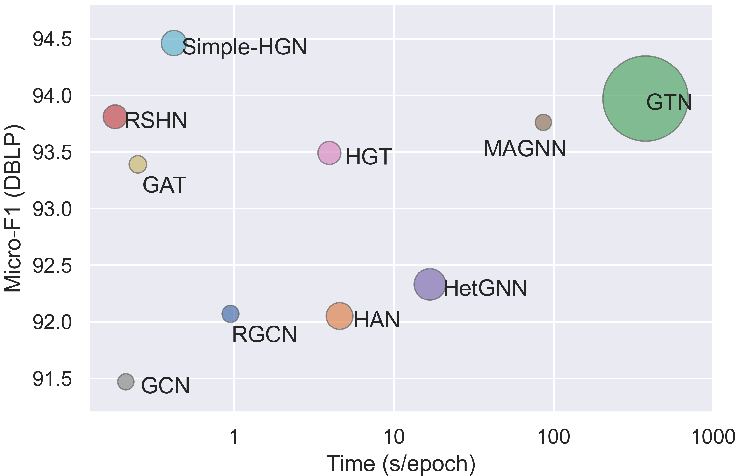
The main drawback of GTN is that it consumes gigantic amount of time and memory. For example, it needs 120 GB memory and 12 hours to train a GTN on DBLP with only 18,000 nodes. In contrast, GCN and GAT only take 1 GB memory and 10 seconds of time.

Moreover, when we test the GTN and GAT five times using the official codes of GTN, we find from Table 1 that their average scores are not significantly different, though GTN consumes $>400\times$ time and $120\times$ memory of GAT.

3.1.3. RSHN (Zhu et al., 2019)

Relation structure-aware heterogeneous graph neural network (RSHN) builds coarsened line graph to obtain edge features first, then uses a novel Message Passing Neural Network (MPNN) (Gilmer et al., 2017) to propagate node and edge features.

The experiments in RSHN have serious problems according to the official code. First, it does not use validation set, and just tune hyperparameters on test set. Second, it reports the accuracy at the epoch with best accuracy on test set in the paper. As shown in Table 1, our well-tuned GAT can even reach 100% accuracy under this improper setting on the AIFB and BGS datasets, which is far better than the 91.67% and 66.32% reported in their paper.

3.1.4. HetGNN (Zhang et al., 2019)

Heterogeneous graph neural network (HetGNN) first uses random walks with restart to generate neighbors for nodes, and then leverages Bi-LSTM to aggregate node features for each type and among types.

HetGNN has the same “information missing in homogeneous baselines” problem as HAN: when comparing it with GAT, a sampled graph instead of the original full graph is fed to GAT. As demonstrated in Table 1, GAT with correct inputs gets clearly better performance.

3.1.5. MAGNN (Fu et al., 2020)

Meta-path aggregated graph neural network (MAGNN) is an enhanced HAN. The motivation is that when HAN deals with meta-path neighbor graphs, it only considers two endpoints of the meta-paths but ignores the intermediate nodes. MAGNN proposes several meta-path encoders to encode all the information along the path, instead of only the endpoints.

However, there are two problems in the experiments of MAGNN. First, MAGNN inherits the “information missing in homogeneous baselines” problem from HAN, and also underperforms GAT with correct inputs.

More seriously, MAGNN has a data leakage problem in link prediction, because it uses batch normalization, and loads positive and negative links sequentially during both training and testing periods. In this way, samples in a minibatch are either all positive or all negative, and the mean and variance in batch normalization will provide extra information. If we shuffle the test set to make each minibatch contains both positive and negative samples randomly, the AUC of MAGNN drops dramatically from 98.91 to 71.49 on the Last.fm dataset.

3.1.6. HGT (Hu et al., 2020a)

Heterogeneous graph transformer (HGT) proposes a transformer-based model for handling large academic heterogeneous graphs with heterogeneous subgraph sampling. As HGT mainly focuses on handling web-scale graphs via graph sampling strategy (Hamilton et al., 2017; Yang et al., 2020a), the datasets used in its paper (¿ 10,000,000 nodes) are unaffordable for most HGNNs, unless adapting them by subgraph sampling. To eliminate the impact of subgraph sampling techniques on the performance, we apply HGT with its official code on the relatively small datasets that are not used in its paper, producing mixed results when compared to GAT (See Table 3).

3.1.7. HetSANN (Hong et al., 2020)

Attention-based graph neural network for heterogeneous structural learning (HetSANN) uses a type-specific graph attention layer for the aggregation of local information, avoiding manually selecting meta-paths. HetSANN is reported to have promising performance in the paper.

However, the datasets and preprocessing details are not released with the official codes, and responses from its authors are not received as of the submission of this work. Therefore, we directly apply HetSANN with standard hyperparameter-tuning, giving unpromising results on other datasets (See Table 3).

3.2. Link Prediction

3.2.1. RGCN (Schlichtkrull et al., 2018)

Relational graph convolutional network (RGCN) extends GCN to relational (multiple edge types) graphs. The convolution in RGCN can be interpreted as a weighted sum of ordinary graph convolution with different edge types. For each node $i$, the $l^{th}$ layer of convolution are defined as follows,

(3) $${𝒉}_i^{(l)}=\sigma \left(\sum _{r\in T_e}\sum _{j\in {𝒩}_i^r}\frac{1}{c_{i,r}}{𝑾}_r^{(l)}{𝒉}_j^{(l)}+{𝑾}_0^{(l)}{𝒉}_i^{(l-1)}\right),$$

where $c_{i,r}$ is a normalization constant and $W_0,W_r$s are learnable parameters.

3.2.2. GATNE (Cen et al., 2019)

General attributed multiplex heterogeneous network embedding (GATNE) leverages the graph convolution operation to aggregate the embeddings from neighbors. It relies on Skip-gram to learn a general embedding, a specific embedding and an attribute embedding respectively, and finally fuses all of them. In fact, GATNE is more a network embedding algorithm than a GNN-style model.

3.3. Knowledge-Aware Recommendation

Recommendation is a main application for Heterogeneous GNNs, but most related works (Fan et al., 2019b, a; Niu et al., 2020; Liu et al., 2020) only focus on their specific industrial data, resulting in non-open datasets and limited transferability of the models. Knowledge-aware recommendation is an emerging sub-field, aiming to improve recommendation by linking items with entities in an open knowledge graph. In this paper, we mainly survey and benchmark models on this topic.

3.3.1. KGCN (Wang et al., 2019d) and KGNN-LS (Wang et al., 2019c)

KGCN enhances the item representation by performing aggregations among its corresponding entity neighborhood in a knowledge graph. KGNN-LS further poses a label smoothness assumption, which posits that similar items in the knowledge graph are likely to have similar user preference. It adds a regularization term to help learn such a personalized weighted knowledge graph.

3.3.2. KGAT (Wang et al., 2019a)

KGAT shares a generally similar idea with KGCN. The main difference lies in an auxiliary loss for knowledge graph reconstruction and the pretrained BPR-MF (Rendle et al., 2009) features as inputs. Although not detailed in its paper, an important contribution of KGAT is to introduce the pretrained features into this tasks, which greatly improves the performance. Based on this finding, we successfully simplify KGAT and obtain similar or even better performance (See Table 5, denoted as KGAT$-$).

3.4. Summary

In summary, the prime common issue of existing HGNNs is the lack of fair comparison with homogeneous GNNs and other works—to some extent—encourage the new models to equip themselves with novel yet redundant modules, instead of focusing more on progress in performance. Additionally, a non-negligible proportion of works have individual issues, e.g., data leakage (Fu et al., 2020), tuning on test set (Zhu et al., 2019), and two-order-of-magnitude more memory and time consumption without effectiveness improvements (Yun et al., 2019).

In light of the significant discrepancy, we take the initiative to setup a heterogeneous graph benchmark (HGB) with these three tasks on diverse datasets for open, reproducible heterogeneous graph research (See §4). Inspired by the promising advantages of the simple GAT over dedicated and relatively-complex heterogeneous GNN models, we present a simple heterogeneous GNN model with GAT as backbone, offering promising results on HGB (See §5).

4. Heterogeneous Graph Benchmark

4.1. Motivation and Overview

Issues with current datasets. Several types of datasets—academic networks (e.g., ACM, DBLP), information networks (e.g., IMDB, Reddit), and recommendation graphs (e.g., Amazon, MovieLens)—are the most frequently-used datasets, but the detailed task settings could be quite different in different papers. For instance, HAN (Wang et al., 2019b) and GTN (Yun et al., 2019) discard the citation links in ACM, while others use the original version. Besides, different splits of the dataset also contribute to uncomparable results. Finally, the recent graph benchmark OGB (Hu et al., 2020c) mostly focuses on benchmarking graph machine learning methods on homogeneous graphs and is not dedicated to heterogeneous graphs.

Issues with current pipelines. To fulfill a task, components outsides HGNNs can also play critical roles. For example, MAGNN (Fu et al., 2020) finds that not all types of node features are useful, and a pre-selection based on validation set could be helpful (See § 4.3). RGCN (Schlichtkrull et al., 2018) uses DistMult (Yang et al., 2014) instead of dot product for training in link prediction. We need to control the other components in the pipeline for fair comparison.

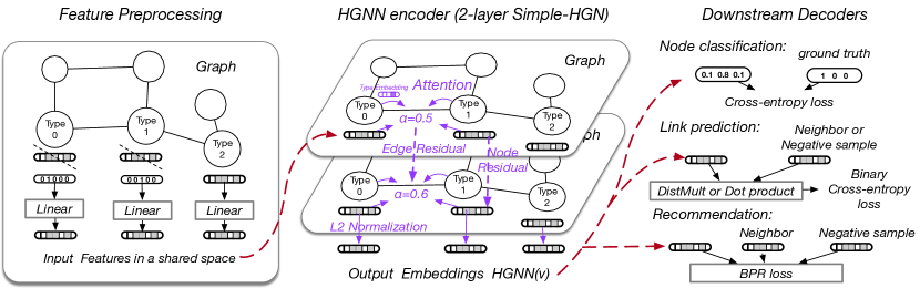
HGB. In view of these practical issues, we present the heterogeneous graph benchmark (HGB) for open, reproducible heterogeneous GNN research. We standardize the process of data splits, feature processing, and performance evaluation, by establishing the HGB pipeline “feature preprocessing $\to$ HGNN encoder $\to$ downstream decoder”. For each model, HGB selects the best fit feature preprocessing and downstream decoder based on its performance on validation set.

4.2. Dataset Construction

HGB collects 11 widely-recognized medium-scale datasets with predefined meta-paths from previous works, making it available to all kinds of HGNNs. The statistics are summarized in Table 2.

4.2.1. Node Classification

Node Classification follows a transductive setting, where all edges are available during training and node labels are split according to 24% for training, 6% for validation and 70% for test in each dataset.

• DBLP is a bibliography website of computer science. We use a commonly used subset in 4 areas with nodes representing authors, papers, terms and venues.

• IMDB is a website about movies and related information. A subset from Action, Comedy, Drama, Romance and Thriller classes is used.

• ACM is also a citation network. We use the subset hosted in HAN (Wang et al., 2019b), but preserve all edges including paper citations and references.

• Freebase (Bollacker et al., 2008) is a huge knowledge graph. We sample a subgraph of 8 genres of entities with about 1,000,000 edges following the procedure of a previous survey (Yang et al., 2020c).

4.2.2. Link Prediction

Link prediction is formulated as a binary classification problem in HGB. The edges are split according to 81% for training, 9% for validation and 10% for test. Then the graph is reconstructed only by edges in the training set. For negative node pairs in testing, we firstly tried uniform sampling and found that most models could easily make a nearly perfect prediction (See Appendix B). Finally, we sample 2-hop neighbors for negative node pairs, of which are 1:1 ratio to the positive pairs in the test set.

• Amazon is an online purchasing platform. We use the subset preprocessed by GATNE (Cen et al., 2019), containing electronics category products with co-viewing and co-purchasing links between them.

• LastFM is an online music website. We use the subset released by HetRec 2011 (Cantador et al., 2011), and preprocess the dataset by filtering out the users and tags with only one link.

• PubMed is a biomedical literature library. We use the subset constructed by HNE (Yang et al., 2020c).

4.2.3. Knowledge-aware recommendation

We randomly split 20% of user-item interactions as test set for each user, and for the left 80% interactions as training set.

• Amazon-book is a subset of Amazon-review related to books.

• LastFM is a subset extracted from last.fm with timestamp from January, 2015 to June, 2015.

• Yelp-2018 is a dataset adapted from 2018 edition of the Yelp challenge. Local businesses like restaurants and bars are seen as items.

• Movielens is a subset of Movielens-20M, which is a widely used dataset for recommendation.

To assure the quality of dataset, we use 10-core setting to filter low-frequency nodes. To align items to knowledge graph entities, we adopt the same procedure as (Wang et al., 2019d, a).

Table 2. Statistics of HGB datasets.

Node Classification	#Nodes	#Node Types	#Edges	#Edge Types	Target	#Classes
DBLP	26,128	4	239,566	6	author	4
IMDB	21,420	4	86,642	6	movie	5
ACM	10,942	4	547,872	8	paper	3
Freebase	180,098	8	1,057,688	36	book	7
Link Prediction					Target
Amazon	10,099	1	148,659	2	product-product
LastFM	20,612	3	141,521	3	user-artist
PubMed	63,109	4	244,986	10	disease-disease

Recommendation	Amazon-book	LastFM	Movielens	Yelp-2018
#Users	70,679	23,566	37,385	45,919
#Items	24,915	48,123	6,182	45,538
#Interactions	846,434	3,034,763	539,300	1,183,610
#Entities	113,487	106,389	24,536	136,499
#Relations	39	9	20	42
#Triplets	2,557,746	464,567	237,155	1,853,704

4.3. Feature Preprocessing

As pointed out in § 4.1, the preprocessing for input features has a great impact on the performance. Our preprocessing methods are as follows.

Linear Transformation. As the input feature of different types of nodes may vary in dimension, we use a linear layer with bias for each node type to map all node features to a shared feature space. The parameters in these linear layers will be optimized along with the following HGNN.

Useful Types Selection. In many datasets, only features of a part of types are useful to the task. We can select a subset of node types to keep their features, and replace the features of nodes of other types as one-hot vectors. Combined with linear transformation, the replacement is equivalent to learn an individual embedding for each node of the unselected types. Ideally, we should enumerate all subsets of types and report the best one based on the performance on the validation set, but due to the high consumption to train the model $2^{|T_v|}$ times, we decide to only enumerate three choices, i.e. using all given node features, using only features of target node type, or replacing all node features as one-hot vectors.

4.4. Downstream Decoders and Loss function

4.4.1. Node Classification

After setting the final dimension of HGNNs the same as the number of classes, we then adopt the most usual loss functions. For single-label classification, we use softmax and cross-entropy loss. For multi-label datasets, i.e. IMDB in HGB, we use a sigmoid activation and binary cross-entropy loss.

4.4.2. Link Prediction

As RGCN (Battaglia et al., 2018) suggests, DistMult (Yang et al., 2014) performs better than direct dot product, due to multiple types of edges, i.e. for node pair $u,v$ and a target edge type $r$,

(4) $${\text{Prob}}_r(u,v\text{is positive})=\text{sigmoid}\left(\text{HGNN}{(u)}^T{R}_r\text{HGNN}(v)\right),$$

where $R_r$ is a learnable square matrix (sometimes regularized with diagonal matrix) for type $r\in T_e$. We find that DistMult outperforms dot product sometimes even when there is only single type of edge to predict. We try both dot product and DistMult decoders, and report the best results. The loss function is binary cross-entropy.

4.4.3. Knowledge-aware Recommendation

Recommendation is similar to link prediction, but differs in data distribution and focuses more on ranking. We define the similarity function $f(u,v)$ between nodes $u,v$ based on dot product. As mentioned in § 3.3.2, pretrained BPR-MF embeddings are of vital importance. We incorporate the BPR-MF embeddings $e_u,e_v$ via a bias term in $f(u,v)$ to avoid modification on the input or architectures of other models, i.e.,

(5) $$f(u,v)=\text{HGNN}{(u)}^T\text{HGNN}(v)+e_u^T{e}_v.$$

Following KGAT (Wang et al., 2019a), we opt for BPR (Rendle et al., 2009) loss for training.

(6) $$\text{Loss}(u,v^{+},v^{-})=-\log \text{sigmoid}\left(f(u,v^{+})-f(u,v^{-})\right),$$

where $(u,v^{+})$ is a positive pair, and $(u,v^{-})$ is a negative pair sampled at random.

Figure 1. HGB pipeline and Simple-HGN. In this illustration, we assume only the features of Type 2 nodes are kept in the Feature Preprocessing period. The purple parts are the improvements over GAT in Simple-HGN.

4.5. Evaluation Settings

We evaluate all methods for all datasets by running 5 times with different random seeds, and reporting the average score and standard deviation.

4.5.1. Node Classification

We evaluate node classification with Macro-F1 and Micro-F1 metrics for both multi-class (DBLP, ACM, Freebase) and multi-label (IMDB) datasets. The implementation is based on sklearn.

4.5.2. Link Prediction

We evaluate link prediction with ROC-AUC (area under the ROC curve) and MRR (mean reciprocal rank) metrics. Since we usually need to determine a threshold when to classify a pair as positive for the score given by decoder, ROC-AUC can evaluate the performance under difference threshold at a whole scope. MRR can evaluate the ranking performance for different methods. Following (Yang et al., 2020c), we calculate MRR scores clustered by the head of pairs in test set, and return the average of them as MRR performance.

4.5.3. Knowledge-aware Recommendation

Recommendation task focuses more on ranking instead of classification. Therefore, we adopt recall@20 and ndcg@20 as our evaluation metrics. The average metrics for all users in test set are reported as benchmark performance.

5. A Simple Heterogeneous GNN

Inspired by the advantage of the simple GAT over advanced and dedicated heterogeneous GNNs, we present Simple-HGN, a simple and effective method for modeling heterogeneous graph. Simple-HGN adopts GAT as backbone with enhancements from the redesign of three well-known techniques: Learnable edge-type embedding, residual connections, and $L_2$ normalization on the output embeddings. Figure 1 illustrates the full pipeline with Simple-HGN .

5.1. Learnable Edge-type Embedding

Though GAT has powerful capacity in modeling homogeneous graphs, it may be not optimal for heterogeneous graphs due to the neglect of node or edge types. To tackle this problem, we extend the original graph attention mechanism by including edge type information into attention calculation. Specifically, at each layer, we allocate a $d_l-$dimensional embedding ${𝒓}_{\psi (e)}^{(l)}$ for each edge type $\psi (e)\in T_e$, and use both edge type embeddings and node embeddings to calculate the attention score as follows:

(7) $${\widehat{\alpha }}_{ij}=\frac{\exp \left(\text{LeakyReLU}\left({𝒂}^T[𝑾{𝒉}_i\Vert 𝑾{𝒉}_j\Vert {𝑾}_r{𝒓}_{\psi (⟨i,j⟩)}]\right)\right)}{{\sum }_{k\in {𝒩}_i}\exp \left(\text{LeakyReLU}\left({𝒂}^T[𝑾{𝒉}_i\Vert 𝑾{𝒉}_k\Vert {𝑾}_r{𝒓}_{\psi (⟨i,k⟩)}]\right)\right)},$$

where $\psi (⟨i,j⟩)$ represents the type of edge between node $i$ and node $j$, and ${𝑾}_r^{(l)}$ is a learnable matrix to transform type embeddings.

Table 3. Node classification benchmark. Vacant positions (“-”) mean that the models run out of memory on large graphs.

	DBLP		IMDB		ACM		Freebase
	Macro-F1	Micro-F1	Macro-F1	Micro-F1	Macro-F1	Micro-F1	Macro-F1	Micro-F1
RGCN	91.52$\pm$0.50	92.07$\pm$0.50	58.85$\pm$0.26	62.05$\pm$0.15	91.55$\pm$0.74	91.41$\pm$0.75	46.78$\pm$0.77	58.33$\pm$1.57
HAN	91.67$\pm$0.49	92.05$\pm$0.62	57.74$\pm$0.96	64.63$\pm$0.58	90.89$\pm$0.43	90.79$\pm$0.43	21.31$\pm$1.68	54.77$\pm$1.40
GTN	93.52$\pm$0.55	93.97$\pm$0.54	60.47$\pm$0.98	65.14$\pm$0.45	91.31$\pm$0.70	91.20$\pm$0.71	-	-
RSHN	93.34$\pm$0.58	93.81$\pm$0.55	59.85$\pm$3.21	64.22$\pm$1.03	90.50$\pm$1.51	90.32$\pm$1.54	-	-
HetGNN	91.76$\pm$0.43	92.33$\pm$0.41	48.25$\pm$0.67	51.16$\pm$0.65	85.91$\pm$0.25	86.05$\pm$0.25	-	-
MAGNN	93.28$\pm$0.51	93.76$\pm$0.45	56.49$\pm$3.20	64.67$\pm$1.67	90.88$\pm$0.64	90.77$\pm$0.65	-	-
HetSANN	78.55$\pm$2.42	80.56$\pm$1.50	49.47$\pm$1.21	57.68$\pm$0.44	90.02$\pm$0.35	89.91$\pm$0.37	-	-
HGT	93.01$\pm$0.23	93.49$\pm$0.25	63.00$\pm$1.19	67.20$\pm$0.57	91.12$\pm$0.76	91.00$\pm$0.76	29.28$\pm$2.52	60.51$\pm$1.16
GCN	90.84$\pm$0.32	91.47$\pm$0.34	57.88$\pm$1.18	64.82$\pm$0.64	92.17$\pm$0.24	92.12$\pm$0.23	27.84$\pm$3.13	60.23$\pm$0.92
GAT	93.83$\pm$0.27	93.39$\pm$0.30	58.94$\pm$1.35	64.86$\pm$0.43	92.26$\pm$0.94	92.19$\pm$0.93	40.74$\pm$2.58	65.26$\pm$0.80
Simple-HGN	94.01$\pm$0.24	94.46$\pm$0.22	63.53$\pm$1.36	67.36$\pm$0.57	93.42$\pm$0.44	93.35$\pm$0.45	47.72$\pm$1.48	66.29$\pm$0.45

Table 4. Link prediction benchmark. Vacant positions (“-”) are due to lack of meta-paths on those datasets.

	Amazon		LastFM		PubMed
	ROC-AUC	MRR	ROC-AUC	MRR	ROC-AUC	MRR
RGCN	86.34$\pm$0.28	93.92$\pm$0.16	57.21$\pm$0.09	77.68$\pm$0.17	78.29$\pm$0.18	90.26$\pm$0.24
GATNE	77.39$\pm$0.50	92.04$\pm$0.36	66.87$\pm$0.16	85.93$\pm$0.63	63.39$\pm$0.65	80.05$\pm$0.22
HetGNN	77.74$\pm$0.24	91.79$\pm$0.03	62.09$\pm$0.01	83.56$\pm$0.14	73.63$\pm$0.01	84.00$\pm$0.04
MAGNN	-	-	56.81$\pm$0.05	72.93$\pm$0.59	-	-
HGT	88.26$\pm$2.06	93.87$\pm$0.65	54.99$\pm$0.28	74.96$\pm$1.46	80.12$\pm$0.93	90.85$\pm$0.33
GCN	92.84$\pm$0.34	97.05$\pm$0.12	59.17$\pm$0.31	79.38$\pm$0.65	80.48$\pm$0.81	90.99$\pm$0.56
GAT	91.65$\pm$0.80	96.58$\pm$0.26	58.56$\pm$0.66	77.04$\pm$2.11	78.05$\pm$1.77	90.02$\pm$0.53
Simple-HGN	93.40$\pm$0.62	96.94$\pm$0.29	67.59$\pm$0.23	90.81$\pm$0.32	83.39$\pm$0.39	92.07$\pm$0.26

Table 5. Knowledge-aware recommendation benchmark. KGAT- refers to KGAT without redundant designs (See § 3.3.2). GCN and GAT are not included, because they are already very similar to KGCN and KGAT-. The KGCN and KGAT works focus more on incorporating knowledge into user-item graphs than new architectures.

	Amazon-Book		LastFM		Yelp-2018		MovieLens
	recall@20	ndcg@20	recall@20	ndcg@20	recall@20	ndcg@20	recall@20	ndcg@20
KGCN	0.1464$\pm$0.0002	0.0769$\pm$0.0002	0.0819$\pm$0.0002	0.0705$\pm$0.0002	0.0683$\pm$0.0003	0.0431$\pm$0.0003	0.4237$\pm$0.0008	0.2753$\pm$0.0005
KGNN-LS	0.1448$\pm$0.0003	0.0759$\pm$0.0001	0.0806$\pm$0.0003	0.0695$\pm$0.0002	0.0671$\pm$0.0003	0.0422$\pm$0.0002	0.4218$\pm$0.0008	0.2741$\pm$0.0005
KGAT	0.1507$\pm$0.0003	0.0802$\pm$0.0004	0.0877$\pm$0.0003	0.0749$\pm$0.0003	0.0697$\pm$0.0002	0.0450$\pm$0.0001	0.4532$\pm$0.0004	0.3007$\pm$0.0008
KGAT$-$	0.1486$\pm$0.0003	0.0790$\pm$0.0002	0.0890$\pm$0.0002	0.0762$\pm$0.0002	0.0715$\pm$0.0001	0.0460$\pm$0.0001	0.4553$\pm$0.0003	0.3031$\pm$0.0006
Simple-HGN	0.1587$\pm$0.0011	0.0854$\pm$0.0005	0.0917$\pm$0.0006	0.0797$\pm$0.0003	0.0732$\pm$0.0003	0.0466$\pm$0.0003	0.4618$\pm$0.0007	0.3090$\pm$0.0007

5.2. Residual Connection

GNNs are hard to be deep due to the over-smoothing and gradient vanishing problems (Li et al., 2018; Xu et al., 2018b). A famous solution to mitigate this problem in computer vision is residual connection (He et al., 2016). However, the original GCN paper (Kipf and Welling, 2017) showed a negative result for residual connection on graph convolution. Recent study (Li et al., 2020) finds that well-designed pre-activation implementation could make residual connection great again in GNNs.

Node Residual. We add pre-activation residual connection for node representation across layers. The aggregation at the $l^{th}$ layer can be expressed as

(8) $${𝒉}_i^{(l)}=\sigma \left(\sum _{j\in {𝒩}_i}{\alpha }_{ij}^{(l)}{𝑾}^{(l)}{𝒉}_j^{(l-1)}+{𝒉}_i^{(l-1)}\right),$$

where ${\alpha }_{ij}^{(l)}$ is the attention weight about edge $⟨i,j⟩$ and $\sigma$ is an activation function (ELU (Clevert et al., 2015) by default). When the dimension changes in the $l-$th layer, an additional learnable linear transformation ${𝑾}_{res}^{(l)}\in {ℝ}^{d_{l+1}\times d_l}$ is needed, i.e.,

(9) $${𝒉}_i^{(l)}=\sigma \left(\sum _{j\in {𝒩}_i}{\alpha }_{ij}^{(l)}{𝑾}^{(l)}{𝒉}_j^{(l-1)}+{𝑾}_{\text{res}}^{(l)}{𝒉}_i^{(l-1)}\right).$$

Edge Residual. Recently, Realformer (He et al., 2020) reveals that residual connection on attention scores is also helpful. After getting the raw attention scores $\widehat{\alpha }$ via Eq. (7), we add residual connections to them,

(10) $${\alpha }_{ij}^{(l)}=(1-\beta ){\widehat{\alpha }}_{ij}^{(l)}+\beta {\alpha }_{ij}^{(l-1)},$$

where hyperparameter $\beta \in [0,1]$ is a scaling factor.

Multi-head Attention. Similar to GAT, we adopt multi-head attention to enhance model’s expressive capacity. Specifically, we perform $K$ independent attention mechanisms according to Equation (8), and concatenate their results as the final representation. The corresponding updating rule is:

(11) $${\alpha }_{ijk}^{(l)}=(1-\beta ){\widehat{\alpha }}_{ijk}^{(l)}+\beta {\alpha }_{ijk}^{(l-1)},$$

(12) $${\widehat{𝒉}}_{ik}^{(l)}=\sum _{j\in {𝒩}_i}{\alpha }_{ijk}^{(l)}{𝑾}_k^{(l)}{𝒉}_j^{(l-1)},$$

(13) $${𝒉}_i^{(l)}=\sigma \left(\underset{k=1}{\overset{K}{\parallel }}{\widehat{𝒉}}_{ik}^{(l)}+{𝑾}_{\text{res}(k)}^{(l)}{𝒉}_i^{(l-1)}\right),$$

where $\parallel$ denotes concatenation operation, and ${\widehat{\alpha }}_{ijk}^{(l)}$ is attention score computed by the $k^{th}$ linear transformation ${𝑾}_k^l$ according to Equation (9).

Usually the output dimension cannot be divided exactly by the number of heads. Following GAT, we no longer use concatenation but adopt averaging for the representation in the final ($L^{th}$) layer, i.e.,

(14) $${𝒉}_i^{(L)}=\frac{1}{K}\sum _{k=1}^K{\widehat{𝒉}}_{ik}^{(L)}.$$

Adaptation for Link Prediction. We slightly modify the model architecture for better performance on link prediction. Edge residual is removed and the final embedding is the concatenation of embeddings from all the layers. This adapted version is similar to JKNet (Xu et al., 2018b).

Table 6. Ablation studies for Simple-HGN.

Task	Node Classification		Link Prediction		Recommendation
Dataset	IMDB		Last.fm		Movielens-20M
Metric	Macro-F1	Micro-F1	ROC-AUC	MRR	recall@20	ndcg@20
Simple-HGN	63.53$\pm$1.36	67.36$\pm$0.57	67.59$\pm$0.23	90.81$\pm$0.32	0.4626$\pm$0.0006	0.3532$\pm$0.0005
w.o. type embedding	63.04$\pm$1.00	67.06$\pm$0.40	67.61$\pm$0.13	90.52$\pm$0.13	0.4632$\pm$0.0005	0.3537$\pm$0.0007
w.o. L2 normalization	58.06$\pm$1.62	65.33$\pm$0.69	61.07$\pm$0.96	82.51$\pm$1.56	0.3837$\pm$0.0187	0.2816$\pm$0.0173
w.o. residual connections	61.61$\pm$2.34	66.28$\pm$1.11	63.33$\pm$0.78	84.13$\pm$0.62	0.4261$\pm$0.0004	0.3192$\pm$0.0006

5.3. $L_2$ Normalization

We find that an $L_2$ normalization on the output embedding is extremely useful, i.e.,

(15) $${𝒐}_i=\frac{{𝒉}_i^{(L)}}{\parallel {𝒉}_i^{(L)}\parallel },$$

where ${𝒐}_i$ is the output embedding of node $i$ and ${𝒉}_i^{(L)}$ is the final representation from Equation (14).

The normalization on the output embedding is very common for retrieval-based tasks, because the dot product will be equivalent to the cosine similarity after normalization. But we also find its improvements for classification tasks, which was also observed in computer vision (Ranjan et al., 2017). Additionally, it suggests to multiply a scaling parameter $\alpha$ to the output embedding (Ranjan et al., 2017). We find that tuning an appropriate $\alpha$ indeed improves the performance, but it varies a lot in different datasets. We thus keep the form of Eq. (15) for simplicity.

6. Experiments

We benchmark results for 1) all HGNNs discussed in Section 3, 2) GCN and GAT, and 3) Simple-HGN on HGB. All experiments are reported with the average and the standard variance of five runs.

6.1. Benchmark

Tables 3, 4, and 5 report results for node classification, link prediction, and knowledge-aware recommendation, respectively. The results show that under fair comparison, 1) the simple homogeneous GAT can matches the best HGNNs in most cases, and 2) inherited from GAT, Simple-HGN consistently outperforms all advanced HGNNs methods for node classification on four datasets, link prediction on three datasets, and knowledge-aware recommendation on three datasets.

Implementations of all previous HGNNs are based on their official codes to avoid errors introduced by re-implementation. The only modification occurs on their data loading interfaces and downstream decoders, if necessary, to make their codes adapt to the HGB pipeline.

We use Adam optimizer with weight decay for all methods, and tune hyperparameters based on the validation set performance. The details of hyperparameters are recorded in Appendix C. For the methods requiring meta-paths, the meta-paths used in benchmark datasets are shown in Appendix D.

6.2. Time and Memory Consumption

We test the time and memory consumption of all available HGNNs for node classification on the DBLP dataset. The results are showed in Figure 2. It is worth noting that we only measure the time consumption of one epoch for each model, but the needed number of epochs until convergence could be various and hard to exactly define. HetSANN is omitted due to our failure to get a reasonable Micro-F1 score.

6.3. Ablation Studies

The ablation studies on all the three tasks are summarized in Table 6. Residual connection and $L_2$ normalization consistently improve performance, but type embedding only slightly boosts the performance on node classification, although it is the best way in our experiments to encode type information explicitly under the GAT framework. We will discuss the possible reasons in § 7.

7. Discussion and Conclusion

In this work, we identify the neglected issues in heterogeneous GNNs, setup the heterogeneous graph benchmark (HGB), and introduce a simple and strong baseline Simple-HGN. The goal of this work is to understand and advance the developments of heterogeneous GNNs by facilitating reproducible and robust research.

Notwithstanding the extensive and promising results, there are still open questions remaining for heterogeneous GNNs and broadly heterogeneous graph representation learning.

Is explicit type information useful? Ablation studies in Table 6 suggest the type embeddings only bring minor improvements. We hypothesize that the main reason is that the heterogeneity of node features already implies the different node and edge types. Another possibility is that the current graph attention mechanism (Veličković et al., 2017) is too weak to fuse the type information with feature information. We leave this question for future study.

Are meta-paths or variants still useful in GNNs? Meta-paths (Sun and Han, 2012) are proposed to separate different semantics with human prior. However, the premise of (graph) neural networks is to avoid the feature engineering process by extracting implicit and useful features underlying the data. Results in previous sections also suggest that meta-path based GNNs do not generate outperformance over the homogeneous GAT. Are there better ways to leverage meta-paths in heterogeneous GNNs than existing attempts? Will meta-paths still be necessary for heterogeneous GNNs in the future and what are the substitutions?

Appendix A Time and Memory Consumption

Figure 2. Time and memory comparison for HGNNs on DBLP. The area of the circles represent the (relative) memory consumption of the corresponding models.

Appendix B Random negative

The distribution of negative samples of test set in link prediction task has a great impact on the performance score. The results with random negative test in our benchmark are shown in Table 7. As we can see, the scores are greater than those in Table 4 by a large margin. Most works (Cen et al., 2019; Fu et al., 2020; Zhang et al., 2019) evaluate link prediction with randomly sampled negative pairs, which are easy to distinguish from the positive pairs for most methods. However, in real world scenarios, we usually need to discriminate positive and negative node pairs with similar characters, instead of random ones, due to the widely used “retrieve then re-rank” industrial pipeline. Therefore, we choose to use sampled 2-hop neighbors as our negative test set in benchmark.

Table 7. Link prediction benchmark with random negative test.

	Amazon		Last.fm		PubMed
	ROC-AUC	MRR	ROC-AUC	MRR	ROC-AUC	MRR
RGCN	89.76$\pm$0.33	95.76$\pm$0.22	81.90$\pm$0.29	96.68$\pm$0.14	88.32$\pm$0.08	96.89$\pm$0.20
GATNE	96.67$\pm$0.08	98.68$\pm$0.06	87.42$\pm$0.22	96.35$\pm$0.24	78.36$\pm$0.92	90.64$\pm$0.49
HetGNN	95.51$\pm$0.39	97.91$\pm$0.08	87.35$\pm$0.02	96.15$\pm$0.18	84.14$\pm$0.01	91.00$\pm$0.03
MAGNN	-	-	76.50$\pm$0.21	85.68$\pm$0.04	-	-
HGT	91.70$\pm$2.31	96.07$\pm$0.68	80.49$\pm$0.78	95.48$\pm$0.38	90.29$\pm$0.68	97.31$\pm$0.09
GCN	98.57$\pm$0.21	99.77$\pm$0.02	84.71$\pm$0.1	96.60$\pm$0.12	86.06$\pm$1.23	98.80$\pm$0.56
GAT	98.45$\pm$0.11	99.61$\pm$0.22	83.55$\pm$2.11	91.45$\pm$5.66	87.57$\pm$1.23	98.38$\pm$0.11
Simple-HGN	98.74$\pm$0.25	99.52$\pm$0.08	91.04$\pm$0.22	99.21$\pm$0.15	91.40$\pm$0.30	96.04$\pm$0.25

Appendix C Hyper-parameters

We search learning rate within $\{1,5\}\times \{{10}^{-6},{10}^{-5},{10}^{-4},{10}^{-3},{10}^{-2}\}$ in all cases, and $\{0,1,2,5\}\times \{{10}^{-6},{10}^{-5},{10}^{-4},{10}^{-3}\}$ for weight decay rate. We set dropout rate as 0.1 in recommendation, and 0.5 in node classification and link prediction by default. For batch size, we will try $\{1024,2048,4096,8192\}$, unless the code of the author has special requirements. For training epoch, we will use early stop mechanism based on the evaluation on validation set to promise fully training.

For brevity, we will denote some variables. Suppose dimension of embeddings for graph layers as $d$, dimension of edge embeddings as $d_e$, dimension of attention vector (if exists) as $d_a$, number of graph layers as $L$, number of attention heads as $n_h$, negative slope of LeakyReLU as $s$.

For input feature type, we use $\text{feat}=0$ to denote using all given features, $\text{feat}=1$ to denote using only target node features, and $\text{feat}=2$ to denote all nodes with one-hot features.

C.1. Simple-HGN

C.1.1. Node classification

We set $d=d_e=64$, $n_h=8$, $\beta =0.05$ for all datasets. For DBLP, ACM and Freebase datasets, we set $L=3$, $s=0.05$. For IMDB dataset, we set $L=6$, $s=0.1$. We set $\text{feat}=0$ for IMDB, $\text{feat}=1$ for ACM, and $\text{feat}=2$ for DBLP and Freebase.

C.1.2. Link prediction

We set $d=64$, $d_e=32$, $n_h=2$, $\beta =0$, $s=0.01$ for all datasets. For Amazon and PubMed, we use DistMult as decoder, and set $L=3$. For LastFM, we use dot product as decoder, and set $L=4$. We use $\text{feat}=2$ for all datasets.

C.1.3. Recommendation

For all datasets, we set $d^{(0)}=64$, $d^{(1)}=32$, $d^{(2)}=16$, $n_h=1$, $s=0.01$ as suggested in (Wang et al., 2019a).

C.2. HAN

C.2.1. Node classification

We set $d=8$, $d_a=128$, $n_h=8$ and $L=2$ for all datasets. For input feature type, we use $\text{feat}=2$ in Freebase, and $\text{feat}=1$ in other datasets. We have also tried larger $d$, but the vairation of performance becoms very large. Therefore, we keep $d=8$ as suggested in HAN’s code.

C.3. GTN

C.3.1. Node classification

We use adaptive learning rate suggested in their paper for all datasets. We set $d=64$, number of GTN channels as 2. For DBLP and ACM, we set $L=2$. For IMDB dataset, we set $L=3$.

Moreover, as suggested in GTN paper, we aggregate the keyword node information as attribute to neighbors and use the left sub-graph to do node classification. We also tried to use the whole graph for GTN. Unfortunately, it collapse in that case, which indicates GTN is sensitive to the graph structure.

C.4. RSHN

For IMDB and DBLP, we set $L=2$ and $d=16$. For ACM, we $L=3$ and $d=32$. We use $\text{feat}=0,1,2$ for ACM, IMDB and DBLP respectively.

C.5. HetGNN

C.5.1. Node classification

We set $d=128$, $\text{feat}=0$, and batch size as 200 for all datasets. For random walk, we set walk length as 30 and the window size as 5.

C.5.2. Link prediction

We set $d=128$, $\text{feat}=2$, and batch size as 200 for all datasets. For random walk, we set walk length as 30 and the window size as 5.

C.6. MAGNN

We set $d=64$, $d_a=128$ and $n_h=8$ in all cases.

C.6.1. Node classification

We use $\text{feat}=1$ in all cases. For DBLP and ACM datasets, we set batch size as 8, and number of neighbor samples as 100. For IMDB dataset, we use full batch training.

C.6.2. Link prediction

We set batch size as 8, and number of neighbor samples as 100 for LastFM. For other datasets, we failed to adapt the MAGNN code to them because there is too much hard-coding.

C.7. HetSANN

C.7.1. Node classification

For ACM, we set $d=64$, $L=3$, $n_h=8$ and $\text{feat}=0$. For IMDB, we set $d=32$, $L=2$, $n_h=4$ and $\text{feat}=1$. For DBLP, we set $d=64$, $L=2$, $n_h=4$ and $\text{feat}=2$.

C.8. HGT

C.8.1. Node Classification

We use layer normalization in each layer, and set $d=64$, $n_h=8$ for all datasets. $L$ is set to 2, 3, 3, 5 for ACM, DBLP, Freebase and IMDB respectively. For input feature type, we use $\text{feat}=2$ in Freebase, $\text{feat}=1$ in IMDB and DBLP, and $\text{feat}=0$ in ACM.

C.8.2. Link Prediction

For all datasets, we use layer normalization in each layer, and set $d=64$, $n_h=8$, $\text{feat}=2$ and DistMult as decoder.

C.9. GCN

C.9.1. Node classification

We set $d=64$ for all datasets. We set $L=3$ for DBLP, ACM and Freebase, and $L=4$ for IMDB. We use $\text{feat}=2$ for DBLP and Freebase, and $\text{feat}=0$ for ACM and IMDB.

C.9.2. Link prediction

We set $d=64$, $L=2$, and $\text{feat}=2$ for all datasets.

C.10. GAT

C.10.1. Node classification

We set $d=64$, $n_h=8$ for all datasets. For DBLP, ACM and Freebase, we set $s=0.05$ and $L=3$. For IMDB, we set $s=0.1$ and $L=5$. We use $\text{feat}=2$ for DBLP and Freebase, $\text{feat}=1$ for ACM, and $\text{feat}=0$ for IMDB.

C.10.2. Link prediction

We set $d=64$, $n_h=4$, $L=3$ and $\text{feat}=2$ for all datasets.

C.11. RGCN

C.11.1. Node classification

We set $L=5$ for all datasets. For ACM, we set $d=16$, $\text{feats}=2$. For DBLP and Freebase, we set $d=16$, $\text{feats}=3$. For IMDB, we set $d=32$, $\text{feats}=1$.

C.11.2. Link prediction

We set $L=4$, $d=64$ and $\text{feat}=2$ for all datasets.

C.12. GATNE

C.12.1. Link prediction

We set $d=200$, $d_e=10$, $d_a=20$, $\text{feat}=2$ for all datasets.

For random walk, we set walk length as 30 and the window size as 5. For neighbor sampling, we set negative samples for optimization as 5, neighbor samples for aggregation as 10.

C.13. KGCN and KGNN-LS

C.13.1. Recommendation

For all datasets, we set $d^{(0)}=64$ and $d^{(1)}=48$. We also tried to stack more graph layers, but performance deteriorates when we do that, which is also found in (Wang et al., 2019d; Wang et al., 2019c) experiments. We use sum aggregator because it has best overall performance as reported in (Wang et al., 2019d).

C.14. KGAT

C.14.1. Recommendation

We set $d^{(0)}=64$, $d^{(1)}=32$, $d^{(2)}=16$ for all datasets. For attention mechanism, we keep the Bi-Interaction aggregator according to their official code.

Appendix D Meta-paths

The meta-paths used in benchmark experiments are shown in Table 8. We try to select meta-paths following prior works. For example, meta-paths in DBLP, IMDB and LastFM are from (Fu et al., 2020). Meta-paths in ACM dataset are based on (Wang et al., 2019b), and we also add some meta-paths related to citation and reference relation, which are not used in (Wang et al., 2019b). For Freebase dataset, we first count the most frequent meta-paths with length from 2 to 4, and then manually select 7 of them according to the performance on validation set.

Table 8. Meta-paths used in benchmark.

Dataset	Meta-path	Meaning
DBLP	APA APTPA APVPA	A: author P: paper T: term V: venue
IMDB	MDM, MAM DMD, DMAMD AMA, AMDMA	M: movie D: director A: actor
ACM	PAP, PSP PcPAP, PcPSP PrPAP, PrPSP	P: paper A: author S: subject c: citation relation r: reference relation
Freebase	BB BFB BLMB BPB BPSB BOFB BUB	B: book F: film L: location M: music P: person S: sport O: organization U: business
LastFM	UU, UAU UATAU AUA, ATA AUUA	U: user A: artist T: tag